By Abby Tomita, undergraduate student, OSU College of Earth, Ocean, and Atmospheric Sciences
From long days in Newport performing the patience-testing task of bomb calorimetry, to spending hours transfixed by the microscopic world that exists in our oceans, I recently got an amazing glimpse into the world of marine biological research working with PhD student Rachel Kaplan. She has been an amazing teacher to my fellow intern Hadley and I, showing us the basics of the research process and introducing us to so many wonderful people at NOAA and the GEMM Lab. I am in my third year studying oceanography here at OSU and had no real lab experience before this, so I was eager to explore this area of research, and not only learn new information about our oceans, but also to see the research process up close and personal.
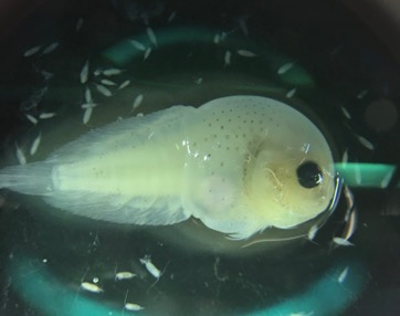
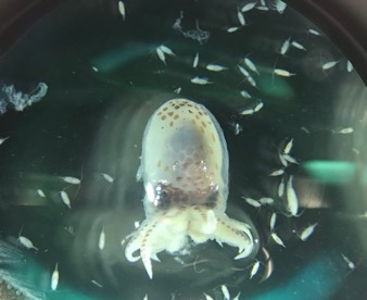
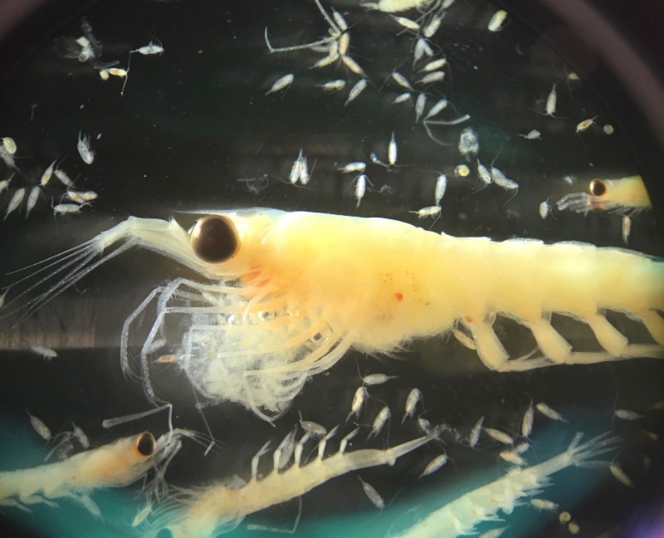
After being trained by Jennifer Fisher, a NOAA Research Fisheries Biologist, I sorted through zooplankton samples collected on the R/V Bell M. Shimada from the Northern California Current region. This data will be used to get an idea of where krill are found throughout the year, and in what abundances. Though my focus was mainly on two species of krill, I also found an assortment of other organisms, such as larval fish, squid, copepods, crabs, and tons of jellies, which were super interesting to see.
A small group of larval squid and other unknown species (photo by Abby Tomita).
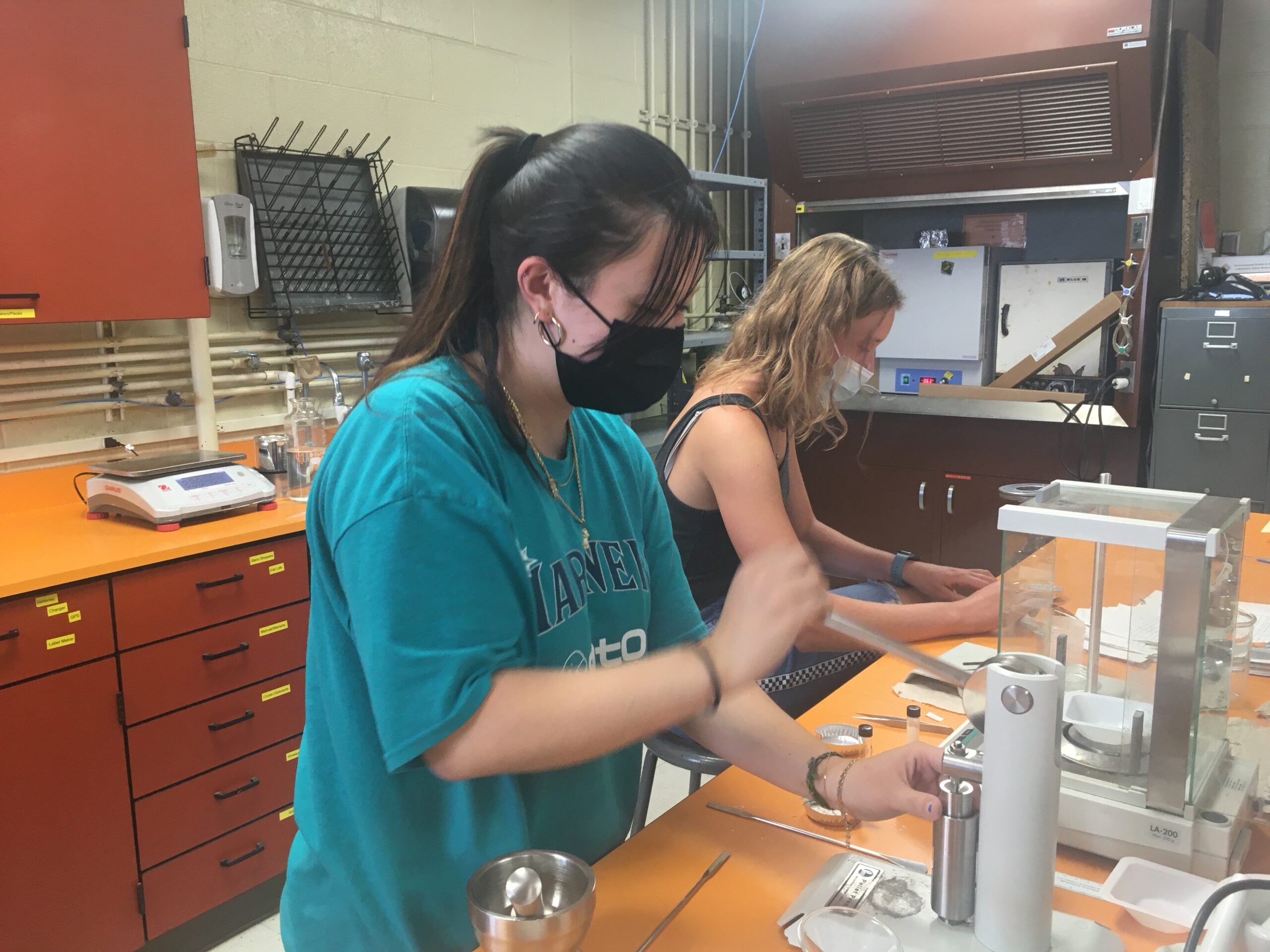
I also studied krill through a technique called bomb calorimetry, which is not for the faint of heart! It takes a tough soul to be able to put these complex little creatures into a mortar and pestle and grind them into a dust that hits your nose like pepper. They then take their final resting place into the bomb calorimetry machine (which can and will find something to fuss over) until it finally manages to ignite and dispose of the krill’s remains. The light that guided me through this dark tunnel was the knowledge that these sacrificial krill were taken in the name of science, with the aim of eventually decreasing whale entanglements.
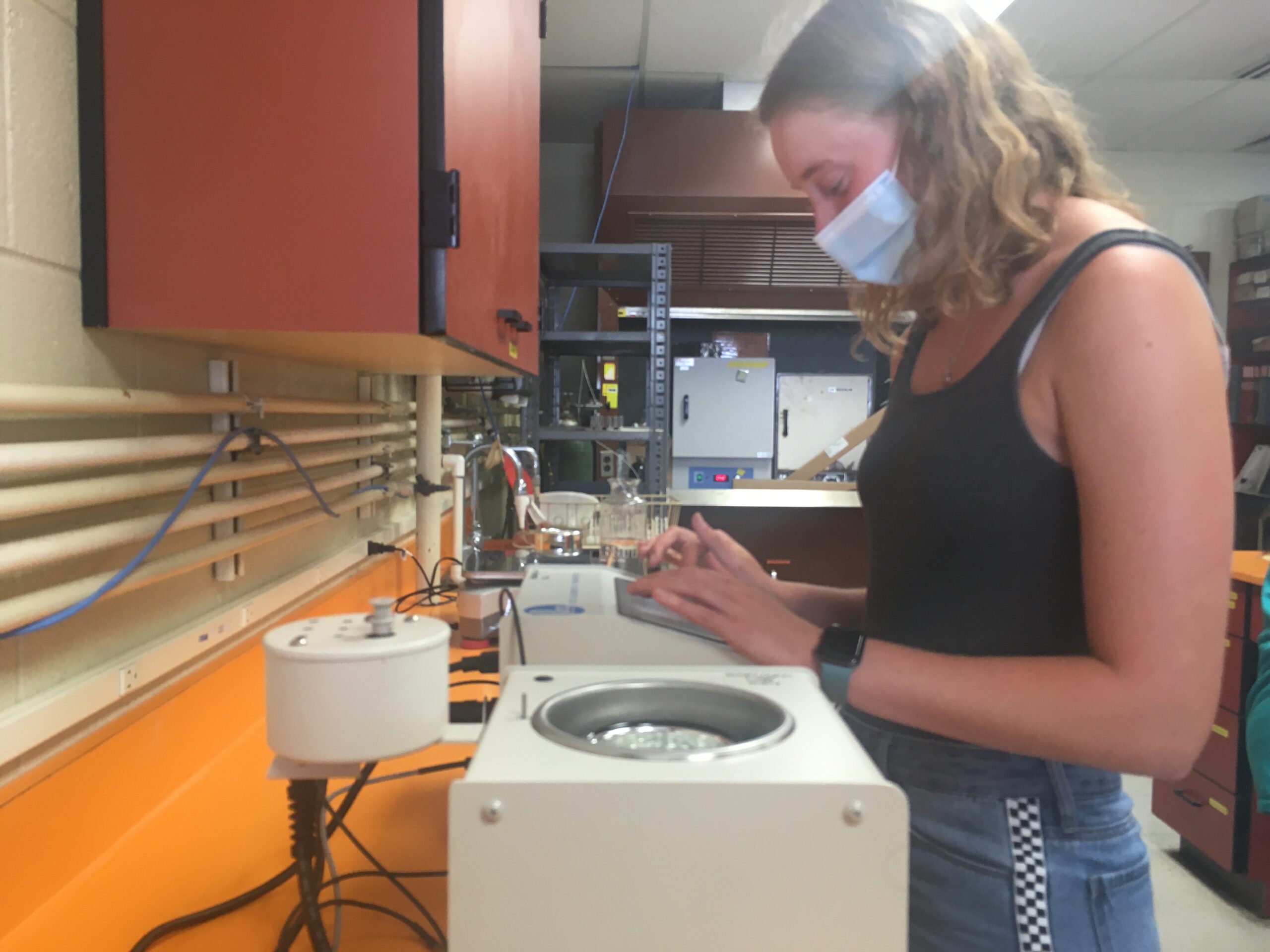
Abby placing the pellet within the coil for the bomb.
That, and Rachel’s contagious positivity. In the early stages, we would spend the majority of our time troubleshooting after constant “misfires”, in which the machine fails to combust the sample properly. Bomb calorimetry involves many tedious steps, and working with such small quantities of tissue – a single krill could weigh 0.01 grams or even less – poses a plethora of its own challenges. One of my biggest takeaways from this experience was to have patience with this kind of work and know when to take a much-needed dance break. Things often do not work out according to plan, and getting to see first-hand how to adapt to confounding variables and hitches in the procedure was an invaluable lesson.
I also got to see how collaborative the research process is. We received helpful advice from other members of the GEMM Lab at lunch, as well as constant help from our esteemed Resident Bomb Cal Expert, Elizabeth Daly. It was comforting for me to see that even when you are doing independent research, you are not expected to only work alone, and there can be so much community in higher level research.
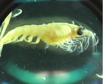
A larval snailfish.A larval fish (sp. unknown) still in its egg.A larval octopus. Female Thysanoessa spinifera krill (photos by Abby Tomita).
Did you enjoy this blog? Want to learn more about marine life, research, and conservation? Subscribe to our blog and get a weekly message when we post a new blog. Just add your name and email into the subscribe box below.
Dr. KC Bierlich, Postdoctoral Scholar, OSU Department of Fisheries, Wildlife, & Conservation Sciences, Geospatial Ecology of Marine Megafauna (GEMM) Lab
Traveling across oceans takes a lot of energy. Most baleen whales use stored energy acquired on their summer foraging grounds to support the costs of migration to and reproduction on their winter breeding grounds. Since little, if any, feeding takes place during the migration and winter season, it is essential that baleen whales obtain enough food to increase their fat reserves to support reproduction. As such, baleen whales are voracious feeders, and they typically depart the foraging grounds much fatter than when they had arrived.
So, how fat do baleen whales typically get by the end of the foraging season, and how does this differ across reproductive classes, such as a juvenile female vs. a pregnant female? Understanding these questions is key for identifying what a typical “healthy” whale looks like, information which can then help scientists and managers monitor potential impacts from environmental and anthropogenic stressors. In this blog, I will discuss a recent publication in Frontiers in Marine Science (https://doi.org/10.3389/fmars.2022.1036860) that is from my PhD dissertation with the Duke University Marine Robotics and Remote Sensing (MaRRS) Lab, and also includes GEMM lab members Allison Dawn and Clara Bird. In this study, we analyzed how humpback whales (Megaptera novaeangliae) along the Western Antarctic Peninsula (WAP) increase their fat reserves throughout the austral summer foraging season (Bierlich et al., 2022). This work also helps provide insight to the GEMM Lab’s GRANITE project (Gray whale Response to Ambient Noise Informed by Technology and Ecology), where we are interested in how Pacific Coast Feeding Group (PCFG) gray whales increase their energy reserves in response to environmental variability and increasing human activities.
Eastern South Pacific humpback whales, identified as Stock G by the International Whaling Commission, travel over 16,000 km between summer foraging grounds along the WAP and winter breeding grounds between Ecuador and Costa Rica (Fig. 1). Like most baleen whales, Stock G humpback whales were heavily exploited by 20th century commercial whaling. Recent evidence suggests that this population is recovering, with an estimated increase in population size of ~7,000 individuals in 2000 to ~19,107 in 2020 (Johannessen et al., 2022).
However, there are long-term concerns for this population. The WAP is one of the fastest warming regions on the planet, and regional populations of krill, an important food source for humpback whales, have declined steeply over the past half-century. Additionally, the WAP has seen a rapid expansion of human activities, such as tourism and krill fishing. Specifically, the WAP has experienced an increase in tourism from a total of 6,700 visitors from 59 voyages in 1990 to 73,000 visitors from 408 voyages in 2020, which may be causing increased stress levels amongst Stock G (Pallin et al., 2022). Furthermore, the krill fishery has increased harvest activities in key foraging areas for humpback whales (Reisinger et al., 2022). Understanding how humpback whales increase their energy reserves over the course of the foraging season can help researchers establish a baseline to monitor future impacts from climate change and human activities. This work also provides an opportunity for comparisons to other baleen whale populations that are also exposed to multiple stressors, such as the PCFG gray whales off the Newport Coast who are constantly exposed to vessel traffic and at risk of entanglement from fishing gear.
Figure 1. The migration route of the Stock G humpback whale population. Figure adapted from Whales of the Antarctic Peninsula Report, WWF 2018.
To understand how humpback whales increase their energy reserves throughout the foraging season, we collected drone imagery of whales along the WAP between November and June, 2017-2019 (Fig. 2). We used these images to measure the length and width of the whale to estimate body condition, which represents an animal’s relative energy reserve and can reflect foraging success (see previous blog). We collected drone imagery from a combination of research stations (Palmer Station), research vessels (Laurence M. Gould), and tour ships (One Ocean Expeditions). We used several different drones types and accounted for measurement uncertainty associated with the camera, focal length lens, altitude, and altimeter (barometer/LiDAR) from each drone (see previous blog and Bierlich et al., 2021a, 2021b). We also took biopsy samples to identify the sex of each individual and to determine if females were pregnant or not.
Figure 2. Two humpbacks gracefully swimming in the chilly water along the Western Antarctic Peninsula. Photo taken by KC Bierlich & the Duke University Marine Robotics and Remote Sensing (MaRRS) Lab.
Our final dataset included body condition measurements for 228 total individuals. We found that body condition increased linearly between November and June for each reproductive class, which included calves, juvenile females, juvenile whales of unknown sex, lactating females, mature whales of unknown sex, and non-pregnant females (Fig. 3). This was an interesting finding because a recent publication analyzing tagged whales from the same population found that humpback whales have high foraging rates in early season that then significantly decrease by February and March (Nichols et al., 2022). So, despite these reduced foraging rates throughout the season, humpback whales continue to gain substantial mass into the late season. This continued increase in body condition implies a change in krill abundance and/or quality into the late season, which may compensate for the lower feeding rates. For example, krill density and biomass increases by over an order of magnitude across the season (Reiss et al., 2017) and their lipid content increases by ~4x (Hagen et al., 1996). Thus, humpback whales likely compensate for their lower feeding rates by feeding on denser and higher quality krill, ultimately increasing their efficiency in energy deposition.
Figure 3. Body condition, here measured as Body Area Index (BAI), increases linearly for each reproductive class across the austral summer foraging season (Nov – June) for humpback whales along the Western Antarctic Peninsula. The shading represents the uncertainty around the estimated relationship. The colors represent the month of data collection.
We found that body condition increase varied amongst reproductive classes. For example, lactating females had the poorest measures of body condition across the season, reflecting the high energetic demands of nursing their calves (Fig. 3). Conversely, non-pregnant females had the highest body condition at the start of the season compared to all the other classes, likely reflecting the energy saved and recovered by skipping breeding that year. Calves, juvenile whales, and mature whales all reached similar levels of body condition by the end of the season, though mature whales will likely invest most of their energy stores toward reproduction, whereas calves and juveniles likely invest toward growth. We also found a positive relationship between the total length of lactating females and their calves, suggesting that bigger moms have bigger calves (Fig. 4). A similar trend has also been observed in other baleen whale species including southern and North Atlantic right whales (Christiansen et al., 2018; Stewart et al., 2022).
Figure 4. Big mothers have big calves. Total length (TL) measurement between mother-calf pairs. The bars around each point represents the uncertainty (95% highest posterior density intervals). The colors represent the month of data collection. The blue line represents the best fit from a Deming regression, which incorporate measurement uncertainty in both the independent (mother’s TL) and dependent variable (calf’s TL).
The results from the humpback study provide insight for my current work exploring how PCFG gray whales increase their energy reserves in relation to environmental variability and increasing human activities. Over the past seven years, the GEMM Lab has been collecting drone images of PCFG gray whales off the coast of Oregon to measure their body condition (see this GRANITE Project blog). Many of the individuals we encounter are seen across years and throughout the foraging season, providing an opportunity to evaluate how an individual’s body condition is influenced by environmental variation, stress levels, maturity, and reproduction. For example, we had nine total body condition measurements of a female PCFG whale named “Sole”, who had a curvilinear increase in body condition throughout the summer foraging season – a rapid increase in early season that slowed as the season progressed (Fig. 5). This raises many questions for us: is this how most PCFG whales typically increase their body condition during the summer? Is this increase different for pregnant or lactating females? How is this increase impacted by environmental variability or anthropogenic stressors? Repeated measurements of individuals, in addition to Sole, in different reproductive classes across different years will help us determine what body condition is considered a healthy range for gray whales. This is particularly important for monitoring any potential health consequences from anthropogenic stressors, such as vessel noise and traffic (see recent blog by GEMM Lab alum Leila Lemos). We are currently analyzing body condition measurements between 2016 – 2022, so stay tuned for upcoming results!
Figure 6. Body condition, here measured as Body Area Index (BAI), increases curvilinearly for “Sole”, a mature female Pacific Coat Feeding Group gray whale, imaged nine times along the Oregon coast in 2021. The colors represent the month of data collection.
References
Bierlich, K. C., Hewitt, J., Bird, C. N., Schick, R. S., Friedlaender, A., Torres, L. G., et al. (2021a). Comparing Uncertainty Associated With 1-, 2-, and 3D Aerial Photogrammetry-Based Body Condition Measurements of Baleen Whales. Front. Mar. Sci. 8, 1–16. doi:10.3389/fmars.2021.749943.
Bierlich, K. C., Hewitt, J., Schick, R. S., Pallin, L., Dale, J., Friedlaender, A. S., et al. (2022). Seasonal gain in body condition of foraging humpback whales along the Western Antarctic Peninsula. Front. Mar. Sci. 9, 1–16. doi:10.3389/fmars.2022.1036860.
Bierlich, K., Schick, R., Hewitt, J., Dale, J., Goldbogen, J., Friedlaender, A., et al. (2021b). Bayesian approach for predicting photogrammetric uncertainty in morphometric measurements derived from drones. Mar. Ecol. Prog. Ser. 673, 193–210. doi:10.3354/meps13814.
Christiansen, F., Vivier, F., Charlton, C., Ward, R., Amerson, A., Burnell, S., et al. (2018). Maternal body size and condition determine calf growth rates in southern right whales. Mar. Ecol. Prog. Ser. 592, 267–281.
Hagen, W., Van Vleet, E. S., and Kattner, G. (1996). Seasonal lipid storage as overwintering strategy of Antarctic krill. Mar. Ecol. Prog. Ser. 134, 85–89. doi:10.3354/meps134085.
Johannessen, J. E. D., Biuw, M., Lindstrøm, U., Ollus, V. M. S., Martín López, L. M., Gkikopoulou, K. C., et al. (2022). Intra-season variations in distribution and abundance of humpback whales in the West Antarctic Peninsula using cruise vessels as opportunistic platforms. Ecol. Evol. 12, 1–13. doi:10.1002/ece3.8571.
Nichols, R., Cade, D. E., Kahane-Rapport, S., Goldbogen, J., Simpert, A., Nowacek, D., et al. (2022). Intra-seasonal variation in feeding rates and diel foraging behavior in a seasonally fasting mammal, the humpback whale. Open Sci. 9, 211674.
Pallin, L. J., Botero-Acosta, N., Steel, D., Baker, C. S., Casey, C., Costa, D. P., et al. (2022). Variation in blubber cortisol levels in a recovering humpback whale population inhabiting a rapidly changing environment. Sci. Rep. 12, 1–13. doi:10.1038/s41598-022-24704-6.
Reisinger, R., Trathan, P. N., Johnson, C. M., Joyce, T. W., Durban, J. W., Pitman, R. L., et al. (2022). Spatiotemporal overlap of baleen whales and krill fisheries in the Antarctic Peninsula region. Front. Mar. Sci. doi:doi: 10.3389/fmars.2022.914726.
Reiss, C. S., Cossio, A., Santora, J. A., Dietrich, K. S., Murray, A., Greg Mitchell, B., et al. (2017). Overwinter habitat selection by Antarctic krill under varying sea-ice conditions: Implications for top predators and fishery management. Mar. Ecol. Prog. Ser. 568, 1–16. doi:10.3354/meps12099.
Stewart, J. D., Durban, J. W., Europe, H., Fearnbach, H., Hamilton, P. K., Knowlton, A. R., et al. (2022). Larger females have more calves : influence of maternal body length on fecundity in North Atlantic right whales. Mar. Ecol. Prog. Ser. 689, 179–189. doi:10.3354/meps14040.
Dr. Alejandro A. Fernández Ajó, Postdoctoral Scholar, Marine Mammal Institute – OSU Department of Fisheries, Wildlife, & Conservation Sciences, Geospatial Ecology of Marine Megafauna (GEMM) Lab.
The English language is recognized as the international language of science (Gordin, 2015); I believe this is a useful convention that allows scientists to communicate ideas and gain access to global scientific literature regardless of their origin or native tongue. However, this avenue for sharing knowledge is open only for those proficient in English, and many scientists and users of scientific information, such as policy makers and conservationists, communicate on a daily basis in languages other than English. This inevitably creates barriers to the transfer of knowledge between communities, potentially impacting conservation and management because scientific knowledge is often unavailable in local languages.
Although in non-English speaking countries, local journals are receptive to publishing scientific research in languages other than English (i.e., their local language), oftentimes these local journals are perceived as low-quality and have a relatively low impact factor, making publishing in such journals less attractive to scientists. Therefore, readers with language barriers only have access to limited studies and are often unaware of the most significant research, even when the research is conducted in their region. This situation can result in a void of information relevant for environmental policies and conservation strategies. Ensuring that research findings are available in the local language of the region in which the research is conducted is an important step in science communication, but one that is often neglected.
In addition, scientists with English as a Foreign Language (EFL) confront the added challenge of navigating a second language while writing manuscripts, preparing and presenting oral presentations, and developing outreach communications (Ramirez-Castaneda, 2020). For example, EFL researchers have reported that one of the primary targets of criticism for their manuscripts under review is often the quality of their English rather than the science itself (Drubin and Kellogg, 2012). In academia, most job interviews and PhD applications are conducted in English; and grant and project proposals are often required to be written in English, which can be particularly challenging and can impact the allocation of resources for research and conservation in non-English speaking regions.
I am from Argentina, and I am a native Spanish speaker. I am fortunate to have started learning English at an early age and continue practicing with international collaborations and traveling abroad. Being able to communicate in English has opened many doors for me, but I recognize that I am in a privileged position with respect to many Argentinians and South Americans in general, where the majority of the population receives minimal training in English and bilingualism with English is very low. Thus, socioeconomic status can influence English proficiency, which then determines scientific success and access to knowledge. I believe that the scientific community should be aware of these issues and work towards improving equality in the process of research collaborations. Providing opportunities for students, and enhancing the availability of scientific knowledge for non-English speaking communities, particularly when the research is relevant for such communities.
In this picture I am with an international group of Fulbright scholars during the Spring International Language Program at the University of Arkansas. This is on of many activities organized by the Fulbright program to create bridges across cultures and languages.
Fortunately, there are several examples pointing towards improving equality in the scientific process, access to knowledge, and opportunities for EFL communities in STEM careers. Several journals are now accepting, or considering to accept the publication of papers in multiple languages. One example of this is the journal Integrative Organismal Biology, which provides the option for publishing the paper abstract in multiple languages. In our recent publication, “Male Bowhead Whale Reproductive Histories Inferred from Baleen Testosterone and Stable Isotopes,” we provided an abstract in five different languages, including Inuktitut, one of primary languages of indigenous groups in the area. And, international exchange programs like the Fulbright Foreign Student Program, of which I was a beneficiary between 2018-2020, enable graduate students and young professionals from abroad to study and conduct research in the United States.
In an effort to contribute to addressing these problems, I am working with a group of colleagues from Argentina (María Constanza (Kata) Marchesi and Tomas Marina) to develop graduate level coursework that will be offered at the Universidad Nacional de la Patagonia in Puerto Madryn, Argentina, with the objective to enable students to learn effective communication using English in the scientific environment. Unfortunately, these types of programs focused on EFL proficiency for STEM students are currently rare in Argentina, but my hope is that our work can spur the creation of additional programs for EFL students in STEM across the region.
I want to finish this post with the acknowledgement of the huge support I have form the GEMM Lab, which welcomes diversity, equity, and inclusivity, and promotes a culture of anti-racism, transparency, and acceptance (See the GEMM Lab DEI statement here).
Did you enjoy this blog? Want to learn more about marine life, research and conservation? Subscribe to our blog and get weekly updates and more! Just add your name into the subscribe box below!
References and Additional Readings
Gordin, M. D. (2015). Scientific Babel : How Science Was Done Before and After Global English. Chicago, IL: University of Chicago Press.
Ramírez-Castañeda V (2020) Disadvantages in preparing and publishing scientific papers caused by the dominance of the English language in science: The case of Colombian researchers in biological sciences. PLoS ONE 15(9): e0238372. https://doi.org/10.1371/journal.pone.0238372
Drubin, D. G., and Kellogg, D. R. (2012). English as the universal language of science: opportunities and challenges. Mol. Biol. Cell 23:1399. doi: 10.1091/mbc.E12-02-0108
Amano, T., González-Varo, J. P., & Sutherland, W. J. (2016). Languages are still a major barrier to global science. PLoS Biology, 14(12), e2000933. https://doi.org/10.1371/journal.pbio.2000933
Marden, E., Abbott, R. J., Austerlitz, F., Ortiz-Barrientos, D., Rieseberg, L. H. (2021). Sharing and reporting benefits from biodiversity research. Molecular Ecology, 30(5), 1103–1107. https://doi.org/10.1111/mec.15702
Márquez, M. C., & Porras, A. M. (2020). Science communication in multiple languages Is critical to Its effectiveness. Frontiers in Communication, 5(May). https://doi.org/10.3389/fcomm.2020.00031
Ramírez-Castañeda V (2020) Disadvantages in preparing and publishing scientific papers caused by the dominance of the English language in science: The case of Colombian researchers in biological sciences. PLoS ONE 15(9): e0238372. https://doi.org/10.1371/journal.pone.0238372
Trisos, C. H., Auerbach, J., & Katti, M. (2021). Decoloniality and anti-oppressive practices for a more ethical ecology. Nature Ecology and Evolution, 5(9), 1205–1212. https://doi.org/10.1038/s41559-021-01460-w
Letter to the Editor of Marine Mammal Science: Enhancing the impact and inclusivity of research by embracing multi-lingual science communication (2022) DOI: 10.13140/RG.2.2.29934.08001 http://dx.doi.org/10.13140/RG.2.2.29934.08001
Leal, J. S., Soares, B., Franco, A. C. S., de Sá Ferreira Lima, R. G., Baker, K., & Griffiths, M. (2022). Decolonizing ecological research: a debate between global North geographers and global South field ecologists. https://doi.org/10.31235/osf.io/wbzh2
Global climate change is affecting all aspects of life on earth. The oceans are not exempt from these impacts. On the contrary, marine species and ecosystems are experiencing significant impacts of climate change at faster rates and greater magnitudes than on land1,2, with cascading effects across trophic levels, impacting human communities that depend on healthy ocean ecosystems3.
In the lobby of the Gladys Valley Marine Studies building that we are privileged to work in here at the Hatfield Marine Science Center, a poem hangs on the wall: “The North Pacific Is Misbehaving”, by Duncan Berry. I read it often, each time moved by how he articulates both the scientific curiosity and the personal emotion that are intertwined in researchers whose work is dedicated to understanding the oceans on a rapidly changing planet. We seek to uncover truths about the watery places we love that capture our fascination; truths that are sometimes beautiful, sometimes puzzling, sometimes heartbreaking. Observations conducted with scientific rigor do not preclude complex human feelings of helplessness, determination, and hope.
Figure 1. Poem by Duncan Berry, entitled, “The North Pacific is Misbehaving”.
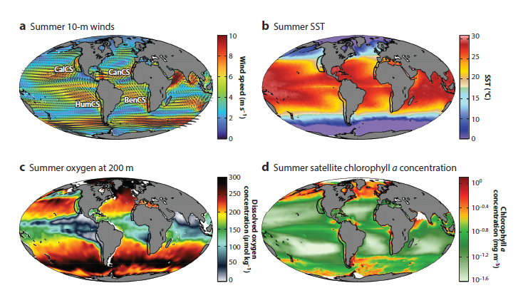
Here on the Oregon Coast, we are perched on the edge of a bountiful upwelling ecosystem. Upwelling is the process by which winds drive a net movement of surface water offshore, which is replaced by cold, nutrient-rich water. When this water full of nutrients meets the sunlight of the photic zone, large phytoplankton blooms occur that sustain high densities of forage species like zooplankton and fish, and yielding important feeding opportunities for predators such as marine mammals. Upwelling ecosystems, like the California Current system in our back yard that features in Duncan Berry’s poem, support over 20% of global fisheries catches despite covering an area less than 5% of the global oceans4–6. These narrow bands of ocean on the eastern boundaries of the major oceans are characterized by strong winds, cool sea surface temperatures, and high primary productivity that ultimately support thriving and productive ecosystems (Fig. 2)7.
Figure 2. Reproduced from Bograd et al. 2023. Maps showing global means in several key properties during the warm season (June through August in the Northern Hemisphere and January through March in the Southern Hemisphere). The locations of the four eastern boundary current upwelling systems (EBUSs) are shown by black outlines in each panel. (a) 10-m wind speed (colors) and vectors. (b) SST. (c) Dissolved oxygen concentrations at 200-m depth. (d) Concentration of ocean chlorophyll a. Abbreviations: BenCS, Benguela Current System; CalCS, California Current System; CanCS, Canary Current System; HumCS, Humboldt Current System; SST, sea surface temperature.
Because of their importance to human societies, eastern boundary current upwelling systems (EBUSs) have been well-studied over time. Now, scientists around the world who have dedicated their careers to understanding and describing the dynamics of upwelling systems are forced to reckon with the looming question of what will happen to these systems under climate change. The state of available information was recently synthesized in a forthcoming paper by Bograd et al. (2023). These authors find that the future of upwelling systems is uncertain, as climate change is anticipated to drive conflicting physical changes in their oceanography. Namely, alongshore winds could increase, which would yield increased upwelling. However, a poleward shift in these upwelling systems will likely lead to long-term changes in the intensity, location, and seasonality of upwelling-favorable winds, with intensification in poleward regions but weakening in equatorward areas. Another projected change is stronger temperature gradients between inshore and offshore areas, and vertically within the water column. What these various opposing forces will mean for primary productivity and species community structure remains to be seen.
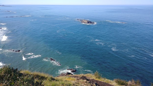
While most of my prior research has centered around the importance of productive upwelling systems for supporting marine mammal feeding grounds8–10, my recent focus has shifted closer to home, to the nearshore waters less than 5 km from the coastline. Despite their ecological and economic importance, nearshore habitats remain understudied, particularly in the context of climate change. Through the recently launched EMERALD project, we are investigating spatial and temporal distribution patterns of harbor porpoises and gray whales between San Francisco Bay and the Columbia River in relation to fluctuations in key environmental drivers over the past 30 years. On a scientific level, I am thrilled to have such a rich dataset that enables asking broad questions relating to how changing environmental conditions have impacted these nearshore sentinel species. On a more personal level, I must admit some apprehension of what we will find. The excitement of detecting statistically significant northward shift in harbor porpoise distribution stands at odds with my own grappling with what that means for our planet. The oceans are changing, and sensitive species must move or adapt to persist. What does the future hold for this “wild edge of a continent of ours” that I love, as Duncan Berry describes?
Figure 4. The view from Cape Foulweather, showing the complex mosaic of nearshore habitat features. Photo: D. Barlow.
Evidence exists that the nearshore realm of the Northeast Pacific is actually decoupled from coastal upwelling processes11. Rather, these areas may be a “sweet spot” in the coastal boundary layer where headlands and rocky reefs provide more stable retention areas of productivity, distinct from the strong upwelling currents just slightly further from shore (Fig. 4). As the oceans continue to shift under the impacts of climate change, what will it mean for these critically important nearshore habitats? While they are adjacent to prominent upwelling systems, they are also physically, biologically, and ecologically distinct. Will nearshore habitats act as a refuge alongside a more rapidly changing upwelling environment, or will they be impacted in some different way? Many unanswered questions remain. I am eager to continue seeking out truth in the data, with my drive for scientific inquiry fueled by my underlying connection to this wild edge of a continent that I call home.
Did you enjoy this blog? Want to learn more about marine life, research, and conservation? Subscribe to our blog and get a weekly alert when we make a new post! Just add your name into the subscribe box below!
References:
1. Poloczanska, E. S. et al. Global imprint of climate change on marine life. Nat. Clim. Chang.3, (2013).
2. Lenoir, J. et al. Species better track climate warming in the oceans than on land. Nat. Ecol. Evol.4, 1044–1059 (2020).
3. Hoegh-Guldberg, O. & Bruno, J. F. The impact of climate change on the world’s marine ecosystems. Science (2010). doi:10.1126/science.1189930
4. Mann, K. H. & Lazier, J. R. N. Dynamics of Marine Ecosystems: Biological-physical interactions in the oceans. Blackwell Scientific Publications (1996). doi:10.2307/2960585
5. Ryther, J. Photosynthesis and fish production in the sea. Science (80-. ).166, 72–76 (1969).
6. Cushing, D. H. Plankton production and year-class strength in fish populations: An update of the match/mismatch hypothesis. Adv. Mar. Biol.9, 255–334 (1990).
7. Bograd, S. J. et al. Climate Change Impacts on Eastern Boundary Upwelling Systems. Ann. Rev. Mar. Sci.15, 1–26 (2023).
8. Barlow, D. R., Bernard, K. S., Escobar-Flores, P., Palacios, D. M. & Torres, L. G. Links in the trophic chain: Modeling functional relationships between in situ oceanography, krill, and blue whale distribution under different oceanographic regimes. Mar. Ecol. Prog. Ser.642, 207–225 (2020).
9. Barlow, D. R., Klinck, H., Ponirakis, D., Garvey, C. & Torres, L. G. Temporal and spatial lags between wind, coastal upwelling, and blue whale occurrence. Sci. Rep.11, 1–10 (2021).
10. Derville, S., Barlow, D. R., Hayslip, C. & Torres, L. G. Seasonal, Annual, and Decadal Distribution of Three Rorqual Whale Species Relative to Dynamic Ocean Conditions Off Oregon, USA. Front. Mar. Sci.9, 1–19 (2022).
11. Shanks, A. L. & Shearman, R. K. Paradigm lost? Cross-shelf distributions of intertidal invertebrate larvae are unaffected by upwelling or downwelling. Mar. Ecol. Prog. Ser.385, 189–204 (2009).
ByRachel Kaplan, PhD student, OSU College of Earth, Ocean and Atmospheric Sciences and Department of Fisheries, Wildlife, & Conservation Sciences, Geospatial Ecology of Marine Megafauna Lab
By Renee Albertson, Senior Instructor and Research Associate, OSU Department of Fisheries, Wildlife, & Conservation Sciences, Marine Mammal Institute
Going to sea is always full of surprises, and the most recent Northern California Current (NCC) cruise was no different. We had surprises both logistical and scientific, disappointing and delightful. By the end, what stood out clearly is that with a great team of people like the one aboard the R/VBell M. Shimada, any challenging situation is made the best of, and any exciting moment is only more so.
Our great science party enjoys the Seattle skyline at the end of the September 2022 NCC cruise.
A few days into the cruise, engine trouble caused the Commanding Officer to decide that we needed to cut the trip short, halt instrument deployment operations, and head in to port. Lucky for us, this new plan included 30 hours of transit to Seattle, and long transits are exactly when we collect marine mammal observations. We were able to keep surveying as we moved up the coast and through the Strait of Juan de Fuca into Seattle. There were many surprises here too – we did not find whales in areas where we have previously sighted many, and overall made fewer sightings than is typical.
For example, we expected to see many whales on the Heceta Head Line (south of Newport), whose shallow depth makes the region a rich underwater garden that supports prey and attracts whales. Instead, we saw hardly any whales in this area. Perhaps they simply weren’t present, or perhaps we missed spotting some whales due to the heavy fog, which makes sighting animals that are not near the ship difficult to impossible. This dearth of animals led us to have to interesting conversations with other researchers as we speculated about what might be going on. The scientists on board these NCC cruises collectively research a wide range of oceanographic fields, including ocean chemistry, phytoplankton, zooplankton, fish, seabirds, and marine mammals. Bringing these data together can provide a better understanding of how the ecosystem is changing over time and help contextualize observations in the moment.
Though we often think about how the distributions of prey structure those of foraging whales, we started to wonder whether a lower trophic level could be at play here. Interestingly, in situ phytoplankton analyses showed a type of diatom called Pseudo-nitzchia along much of our cruise track, with the highest concentration off Cape Meares. In stressful conditions, these diatoms sometimes produce the toxin domoic acid, and we wondered whether this could possibly be related to the low whale counts.
Cells of Pseudo-nitzschia, a genus of microalgae that includes several species that make the neurotoxin domoic acid. NOAA photo courtesy of Vera Trainer.
Along the northern Oregon coast and near the Columbia River, the number of whales we observed increased dramatically. The vast majority were humpbacks, some of which were quite active, breaching and tail slapping the surface of the water. On our best day, we turned into the Strait of Juan de Fuca and sighted about 20 whales in quick succession, as well as a sea otter, and both Steller and California sea lions.
Simultaneously as we surveyed for whales, we were able to continue collecting concurrent echosounder data, which reveals the presence of nearby prey like krill and forage fish. Early in the trip, other researchers also collected krill samples that we could bring back to shore and analyze for their caloric content. Even with a shorter time at sea, we felt lucky to be able to fulfill these scientific goals.
Research cruises always center around two things: science and people. Discussing the scientific surprises we observed with other researchers aboard was inspirational, and left us with interesting questions to pursue. Navigating changes to the cruise plan highlighted the importance of the people aboard even more. Everyone worked together to refine our plans with cooperation and positivity, and we all marveled at what a great group it was, often saying, “Good thing we like each other!”
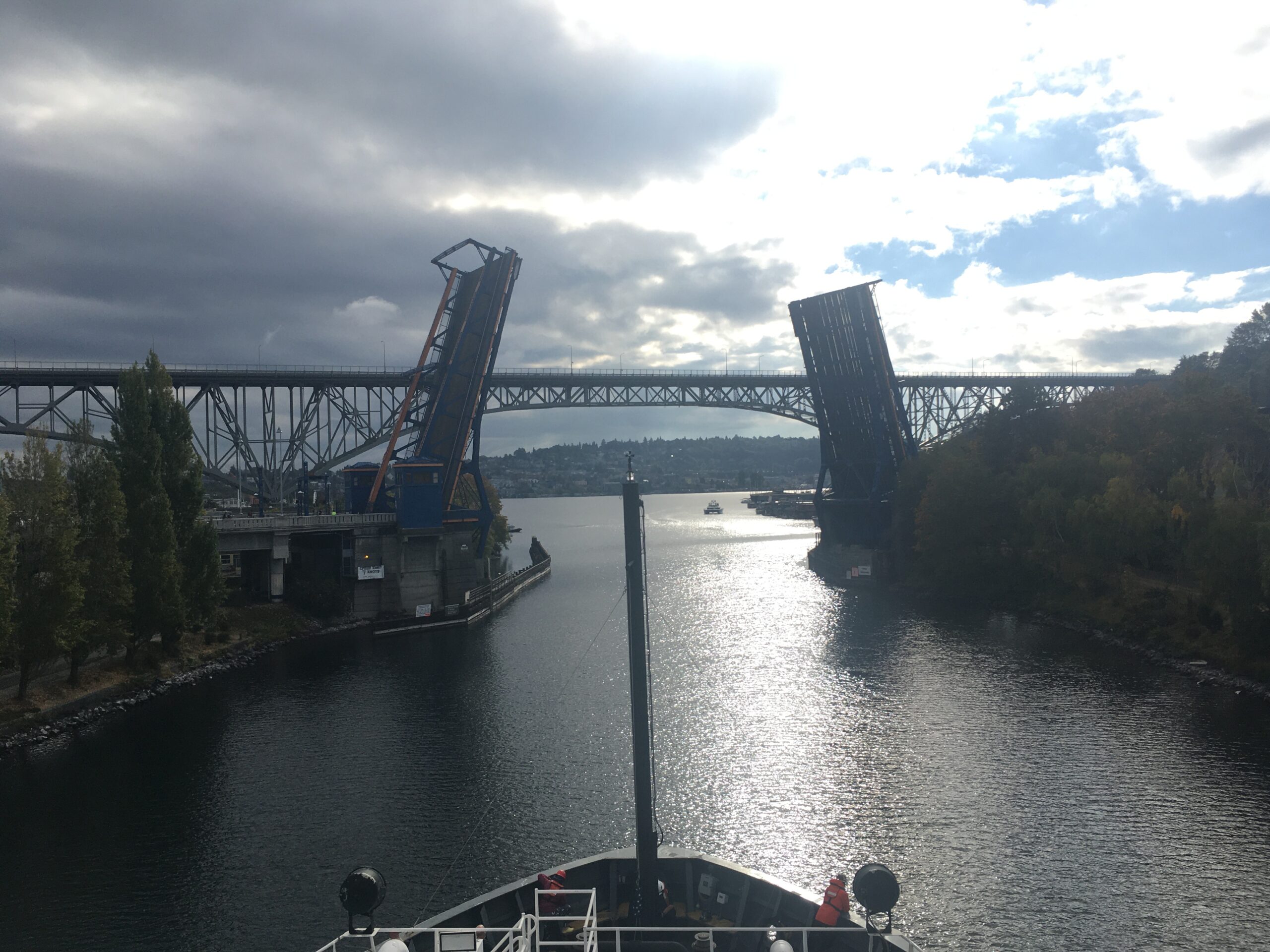
The cruise ended by transiting under the Fremont Bridge into Lake Union.
On the last day of the cruise, we transited into Seattle, moving through the Ballard Locks and into Lake Union. It was an incredible experience to see the city from the water, and an amazing way to cap off the trip. With the next NCC cruise ahead in a few months, we are excited to get back out to sea together soon and tackle whatever surprises come our way.
Did you enjoy this blog? Want to learn more about marine life, research, and conservation? Subscribe to our blog and get a weekly message when we post a new blog. Just add your name and email into the subscribe box below.
By Hadley Robinson, undergraduate student, OSU College of Earth, Ocean, and Atmospheric Sciences and School of Language, Culture, and Society
My name is Hadley Robinson and I am a sophomore undergraduate at OSU, double majoring in Environmental Science and Spanish. This summer, I had the privilege of working with Rachel on her PhD research project involving bomb calorimetry, a technique that allows you to quantify the caloric content of organisms like the zooplankton krill.
Hadley preparing the bomb calorimetry machine to run a sample (photo by Rachel Kaplan).
Prior to this internship, I had never worked in a lab before, and as an environmental science major, I had no previous exposure to oceanography. The connection that Rachel made between our labwork and the broader goal of helping decrease whale entanglement events sparked my interest in this project. Our work this summer aimed to process a set of krill samples collected off the coast of Oregon and Washington, so that we could find the number of calories in single krill, and then look at patterns in krill caloric content based on their species, sex, and other characteristics.
We first identified the krill by species and sex (this was my favorite part of the experiment!). I not only loved looking at them under the microscope, but I also loved how it became a collaborative process. We quickly began getting each other’s opinions on whether or not a krill was Euphausia pacifica, Thysanoessa spinifera, male, female, sexless, gravid (carrying eggs), and much more.
Female Thysanoessa spinifera krill (photo by Abby Tomita).
After identification, we weighed and dried the krill, and finally turned them into small pellets that could fit in an instrument called a bomb calorimeter. These pellets were placed individually into in a “bomb cell” that could then be filled with oxygen and receive a shock from a metal wire. When the machine sent an electric pulse through the wire and combusted the krill pellet, the water surrounding the bomb cell warmed very slightly. The instrument measures this minute temperature change and uses it to calculate the amount of energy in the combusted material. With this information, we were able to quantify how many calories each krill sample contained. Eventually, this data could be used to create a seasonal caloric map of the ocean. Assuming that foraging whales seek out regions with calorically dense prey, such a map could play a crucial role in predicting whale distributions.
Working with Rachel taught me how dynamic the world of research really is. There were many variables that we had to control and factor into our process, such as the possibility of high-calorie lipids being lost if the samples became too warm during the identification process, the risk of a dried krill becoming rehumidified if it sat out in the open air, and even the tiny amount of krill powder inevitably lost in the pelletization process. This made me realize that we cannot control everything! Grappling with these realities taught me to think quickly, adapt, and most importantly, realize that it is okay to refine the process of research as it is being conducted.
Intern Abby (left) pressing the krill powder into a pellet and Hadley (right) prepping the bomb (photo by Rachel Kaplan).
Did you enjoy this blog? Want to learn more about marine life, research, and conservation? Subscribe to our blog and get a weekly message when we post a new blog. Just add your name and email into the subscribe box below.
When I was younger, I aspired to be a marine mammal biologist. I thought it was purely about knowing as much about marine mammal species as possible. However, over time and with experience in this field, I have realized that in order to understand a species, you need to have a holistic understanding of its prey, habitat, and environment. When I first applied to be advised by Leigh in the GEMM Lab, I had no idea how much of my time I would spend looking at tiny zooplankton under a microscope, thinking about the different benefits of different habitat types, or reading about oceanographic processes. But these things have been incredibly vital to my research to date and as a result, I now refer to myself as a marine ecologist. This holistic understanding that I am gaining will only grow throughout my PhD as I am broadly looking at the habitat use, site fidelity, and population dynamics of the Pacific Coast Feeding Group (PCFG) of gray whales for my thesis research.
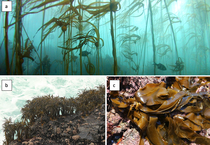
The PCFG display many foraging tactics and occupy several habitat types along the Oregon coast while they spend their summer feeding seasons here (Torres et al. 2018). Here, I will focus on one of these habitats: kelp. When you hear the word kelp, you probably conjure an image of long, thick stalks that reach from the ocean floor to the surface, with billowing fronds waving around (Figure 1a). However, this type is only one of three basic morphologies (Filbee-Dexter & Scheibling 2014) and it is called canopy kelp, which often forms extensive forests. The other two morphologies are stipitate and prostrate kelps. The former forms midwater stands (Figure 1b) while the latter forms low-lying kelp beds (Figure 1c). All three of these morphologies exist on the Oregon coast and create a mosaic of understory and canopy kelp patches that dot our coastline.
Figure 1. Examples of the three different kelp morphologies. a: bull kelp (Nereocystis luetkeana) is a type of canopy kelp and the dominant kelp on the Oregon coast (Source: Oregon Coast Aquarium); b: sea palm (Postelsia palmaeformis) is a type of stipitate kelp that forms mid-water stands (Source: Oregon Conservation Strategy); c: sea cabbage (Saccharina sessilis) is a type of prostrate kelp that is stipeless and forms low-lying kelp beds (Source: Central Coast Biodiversity).
One of the most magnificent things about kelp is that it is not just a species itself, but it provides critical habitat, refuge, and food resources to a myriad of other species due to its high rates of primary production (Dayton 1985). Kelp is often referred to as a foundation species due to all of these critical services it provides. In Oregon, many species of rockfish, which are important commercial and recreational fisheries, use kelp as habitat throughout their life cycle, including as nursery grounds. Lingcod, another widely fished species, forages amongst kelp. A large number of macroinvertebrates can be found in Oregon kelp forests, including anemones, limpets, snails, sea urchins, sea stars, and abalone, to name a fraction of them.
Kelps grow best in cold, nutrient-rich waters (Tegner et al. 1996) and their growth and distribution patterns are highly naturally variable on both temporal and spatial scales (Krumhansl et al. 2016). However, warm water, low nutrient or light conditions, intensive grazing by herbivores, and severe storm activity can lead to the erosion and defoliation of kelp beds (Krumhansl et al. 2016). While these events can occur naturally in cyclical patterns, the frequency of several of these events has increased in recent years, as a result of climate change and anthropogenic impacts. For example, Dawn’s blog discussed increasing marine heatwaves that represent an influx of warm water for a prolonged period of time. In fact, kelps can be useful sentinels of change as they tend to be highly responsive to changes in environmental conditions (e.g., Rogers-Bennet & Catton 2019) and their nearshore, coastal location directly exposes them to human activities, such as pollution, harvesting, and fishing (Bennett et al. 2016).
Due to its foundational role, changes or impacts to kelp can reverberate throughout the ecosystem and negatively affect many other species. As mentioned previously, kelp is naturally highly variable, and like many other ecological processes, undergoes boom and bust cycles. For over four decades, dense, productive kelp forests have been shown to transition to sea urchin barrens, and back again, in natural cycles (Sala et al. 1998;Pinnegar et al. 2000;Steneck et al. 2002; Figure 2). These transitions are called phase shifts. In a healthy, balanced kelp forest, sea urchins typically passively feed on detrital plant matter, such as broken off pieces of kelp fronds that fall to the seafloor. A phase shift occurs when the grazing intensity of sea urchins increases, resulting in them actively feeding on kelp stalks and fronds to a point where the kelp in an area can become greatly reduced, creating an urchin barren. Sea urchin grazing intensity can change for a number of reasons, including reduction in sea urchin predators (e.g., sea otters, sunflower sea stars) or poor kelp recruitment events (e.g., due to warm water temperature). Regardless of the reason, the phases tend to transition back and forth over time. However, there is concern that sea urchin barrens may become an alternative stable state of the subtidal ecosystem from which kelp in an area cannot recover (Filbee-Dexter & Scheibling 2014).
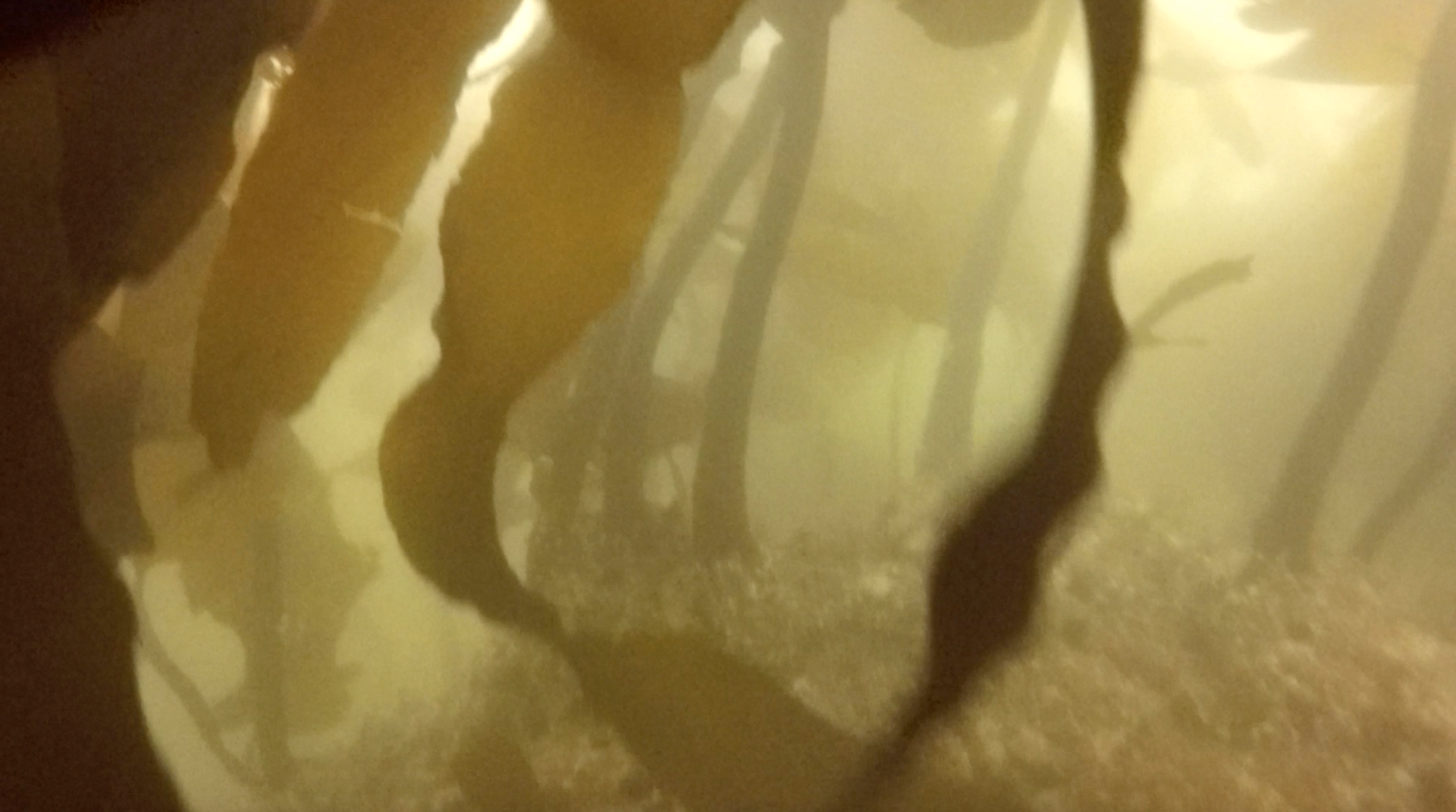
Figure 2. Screenshots from GoPro videos from 2016 (left) and 2018 (right) at the same kayak sampling station in Port Orford showing the difference between a dense kelp forest and what appears to be an urchin barren. (Source: GEMM Lab).
For example, in 2014, bull kelp canopy cover in northern California was reduced by >90% and has not shown signs of recovery since (Rogers-Bennet & Catton 2019; Figure 3). This massive decline was attributed to two major events: 1) the onset of sea star wasting disease (SSWD) in 2013 and 2) the “warm blob” of 2014-2016. SSWD affected over 20 sea star species along the coast from Mexico to Alaska, with the predatory sunflower sea star, which consumes purple sea urchins, most affected, including population declines of 80-100% along the coast (Harvell et al. 2019). Following this SSWD outbreak, the “warm blob”, which was an extreme marine heatwave in the Pacific Ocean, caused ocean temperatures to spike. These two events allowed purple sea urchin populations to grow unchecked by their predators, and created nutrient-poor and warm water conditions, which limited kelp growth and productivity. Intense grazing on bull kelp by growing urchin populations resulted in the >90% reduction in bull kelp canopy cover and has left behind widespread urchin barrens instead (Rogers-Bennet & Catton 2019). Consequently, there have been ecological and economic impacts on the ecosystem and communities in northern California. Without bull kelp, red abalone and red sea urchin populations starved, leading to a subsequent loss of the recreational red abalone (estimated value of $44 million/year) and commercial red urchin fisheries in northern California (Rogers-Bennet & Catton 2019).
Figure 3. Surface kelp canopy area pre- and post-impact from sites in Sonoma and Mendocino counties, northern California from aerial surveys (2008, 2014-2016). Figure and figure caption taken from Rogers-Bennett & Catton (2019).
As I mentioned earlier, while phase shifts between kelp forests and urchin barrens are common cycles, the intensity of the events described above in northern California are an example of sea urchin barrens potentially becoming a stable state of the subtidal ecosystem (Filbee-Dexter & Scheibling 2014). Given that marine heatwaves are only expected to increase in intensity and frequency in the future (Frölicher et al. 2018), the events documented in northern California may not be an isolated incidence.
Considering that parts of the Oregon coast, particularly the southern portion, are very similar to northern California biogeographically, and that it was not exempt from the “warm blob”, similar changes in kelp forests may be occurring along our coast. There are many individuals and groups that are actively working on this issue to examine potential impacts to kelp and the species that depend on the services it provides. For more information, check out the Oregon Kelp Alliance.
Figure 4. A gray whale surfaces in a large kelp bed during a foraging bout along the Oregon coast. (Source: GEMM Lab).
So, what does all of this information have to do with gray whales? Given their affinity for kelp habitats (Figure 4) and their zooplankton prey that aggregates there, changes to kelp ecosystems may affect gray whale health and ecology. This aspect of the complex kelp trophic web has not been examined to date; thus one of my PhD chapters focuses on the response of gray whales to changing kelp ecosystems along the southern Oregon coast. To do this, I am examining 6 years of data collected during the TOPAZ/JASPER project in Port Orford, to look at the relationships between kelp health, sea urchin density, zooplankton abundance, and gray whale foraging effort over space and time. Documenting impacts of changing kelp forests on gray whales is important to assist management efforts as healthy and abundant kelp seems critical in providing ample food opportunities for these iconic Pacific Northwest marine predators.
Did you enjoy this blog? Want to learn more about marine life, research, and conservation? Subscribe to our blog and get a weekly alert when we make a new post! Just add your name into the subscribe box on the left panel.
References
Bennett S, et al. The ‘Great Southern Reef’: Social, ecological and economic value of Australia’s neglected kelp forests. Marine and Freshwater Research 67:47-56.
Dayton PK (1985) Ecology of kelp communities. Annual Review of Ecology and Systematics 16:215-245.
Filbee-Dexter K, Scheibling RE (2014) Sea uechin barrens as alternative stable states of collapsed kelp ecosystems. Marine Ecology Progress Series 495:1-25.
Frölicher TL, Fischer EM, Gruber N (2018) Marine heatwaves under global warming. Nature 560:360-364.
Harvell CD, et al. (2019) Disease epidemic and a marine heat wave are associated with the continental-scale collapse of a pivotal predator (Pycnopodia helianthoides). Science Advances 5(1) doi:10.1126/sciadv.aau7042.
Krumhansl KA, et al. (2016) Global patterns of kelp forest change over the past half-century. Proceedings of the National Academy of Sciences of the United States of America 113(48):13785-13790.
Pinnegar JK, et al. (2000) Trophic cascades in benthic marine ecosystems: lessons for fisheries and protected-area management. Environmental Conservation 27:179-200.
Rogers-Bennett L, Catton CA (2019) Marine heat wave and multiple stressors tip bull kelp forest to sea urchin barrens. Scientific Reports 9:15050.
Sala E, Boudouresque CF, Harmelin-Vivien M (1998) Fishing, trophic cascades and the structure of algal assemblages; evaluation of an old but untested paradigm. Oikos 82:425-439.
Steneck RS, et al. (2002) Kelp forest ecosystems: biodiversity, stability, resilience and future. Environmental Conservation 29:436-459.
Tegner MJ, Dayton PK, Edwards PB, Riser KL (1996) Is there evidence for the long-term climatic change in southern California kelp forests? California Cooperative Oceanic Fisheries Investigations Report 37:111-126.
Torres LG, Nieukirk SL, Lemos L, Chandler TE (2018) Drone up! Quantifying whale behavior from a new perspective improves observational capacity. Frontiers in Marine Science doi:10.3389/fmars.2019.00319.
I wrote my last blogpost in the midst of winter and feeling overwhelmed as I was trying to fly to the US at the peak of the omicron pandemic… Since then, morale has improved exponentially. I have spent two months in the company of my delightful GEMM lab friends, nerding over statistics, sharing scientific conversations, drinking (good!) beer and enjoying the company of this great group of people. During that stay, I was able to focus on my OPAL project more than I have ever been able to, as I set myself the goal of not getting distracted by anything else during my stay in Newport.
The only one distraction that I do not regret is a post I read one morning on the Cetal Fauna Facebook page, a group of cetacean experts and lovers who share news, opinions, photos… anything cetacean related! Someone was posting a photo of a humpback whale stranded in the 1990s’ on Coolum beach, on the east coast of Australia, which is known as a major humpback whale migratory corridor. The story said that (probably with considerable effort) the whale was refloated by many different individuals and organizations present at the beach on that day, specifically Sea World Research, Rescue & Conservation.
I felt very touched by this story and the photo that illustrated it (Figure 1). Seeing all these people come together in this risky operation to save this sea giant is quite something. And the fact that they succeeded was even more impressive! Indeed, baleen whales strand less commonly than toothed whales but their chances of survival when they do so are minimal. In addition to the actual potential damages that might have caused the whale to strand in the first place (entanglements, collisions, diseases etc.), the beaching itself is likely to hurt the animal in a permanent way as their body collapses under their own weight usually causing a cardiovascular failure (e.g., Fernández et al., 2005). The rescue of baleen whales is also simply impaired by the sheer size and weight of these animals. Compared to smaller toothed whales such as pilot whales and false killer whales that happen to strand quite frequently over some coastlines, baleen whales are almost impossible to move off the beach and getting close to them when beached can be very dangerous for responders. For these reasons, I found very few reports and publications mentioning successful rescues of beached baleen whales (e.g., Priddel and Wheeler, 1997; Neves et al., 2020).
Figure 1: Stranded humpback whale on Coolum Beach, East Australia, in 1996. Look at the size of the fluke compared to the men who are trying to rescue her! Luckily, that risky operation ended well. This image won Australian Time Magazine Cover of the year. Credit: Sea World Research, Rescue and Conservation. Photo posted by P. Garbett on https://www.facebook.com/groups/CetalFauna – February 26, 2022)
Now the story gets even better… the following day I received an email from Ted Cheeseman, director and co-founder of Happywhale, a collaborative citizen science tool to share and match photographes of cetaceans (initially only humpback whales but has extended to other species) to recognize individuals based on the unique patterns of the their fluke or dorsal fin. The fluke of the whale stranded in Australia in 1991 had one and only match within the Happywhale immense dataset… and that match was to a whale seen in New Caledonia (Figure 2). “HNC338” was the one!
Figure 2: Happy whale page showing the match of HNC338 between East Australia and New Caledonia. https://happywhale.com/individual/78069;enc=284364?fbclid=IwAR1QEG_6JkpH_k2UrF-qp-9qrOboHYakKjlTj0lLbDFygjN5JugkkKVeMQw
Since I conducted my PhD on humpback whale spatial ecology in New Caledonia, I have continued working on a number of topics along with my former PhD supervisor, Dr Claire Garrigue, in New Caledonia. Although I do not remember each and every whale from her catalogue (composed of more than 1600 humpback whales as of today), I do love a good “whale tale” and I was eager to know who this HNC338 was. I quickly looked into Claire’s humpback whale database and sure enough I found it there: encountered at the end of the 2006 breeding season on September 12th, at a position of 22°26.283’S and 167°01.991’E and followed for an hour. Field notes reported a shy animal that kept the boat at a distance. But most of all, HNC338 was genetically identified as a female and was accompanied by a calf during that season! The calf was particularly big, as expected at this time of the season. What an inspiring thing to think that this whale, stranded in 1996, was resighted 10 years later in a neighboring breeding ground, apparently healthy and raising a calf of her own.
As genetic paternity analysis have been conducted on many New Caledonia calf biopsy samples as part of the Sexy Singing project conducted with our colleagues from St Andrews University in Scotland, we might be able to identify the calf’s father in this breeding stock. Thanks to the great amount of data shared and collected through Happywhale, we are discovering more and more about whale migratory patterns and behavior. It might as well be that this calf’s father was one of those whales that seem to roam over several different breeding grounds (New Caledonia and East Australia). This story is far from finished…
Figure 3: A (pretty bad!) photo of HNC338’s fluke. Luckily the Happywhale matching algorithm is very efficient and was able to detect the similarities of the fluke’s trailing edge compared to figure 1 (Cheeseman et al., 2021). Also of note, see that small dorsal fin popping out of the waters behind big mama’s fluke? That’s her calf!
From the people who pulled this whale back into the water in 1996, to the scientists and cetacean enthusiasts who shared their data and whale photos online, this story once again shows us that hope lies in cooperation! Happywhale was only created in 2015 but since then it has brought together the general public and the scientists to contribute over 465,000 photos allowing the identification of 75,000 different individuals around the globe. In New Caledonia, in Oregon and elsewhere, I hope that these collective initiatives grow more and more in the future, to the benefit of biodiversity and people.
Did you enjoy this blog? Want to learn more about marine life, research, and conservation? Subscribe to our blog and get weekly updates and more! Just add your name into the subscribe box on the left panel.
References
Cheeseman, T., Southerland, K., Park, J., Olio, M., Flynn, K., Calambokidis, J., et al. (2021). Advanced image recognition: a fully automated, high-accuracy photo-identification matching system for humpback whales. Mamm. Biol. doi:10.1007/s42991-021-00180-9.
Fernández, A., Edwards, J. F., Rodríguez, F., Espinosa De Los Monteros, A., Herráez, P., Castro, P., et al. (2005). “Gas and fat embolic syndrome” involving a mass stranding of beaked whales (Family Ziphiidae) exposed to anthropogenic sonar signals. Vet. Pathol. 42, 446–457. doi:10.1354/vp.42-4-446.
Neves, M. C., Neto, H. G., Cypriano-Souza, A. L., da Silva, B. M. G., de Souza, S. P., Marcondes, M. C. C., et al. (2020). Humpback whale (megaptera novaeangliae) resighted eight years after stranding. Aquat. Mamm. 46, 483–487. doi:10.1578/AM.46.5.2020.483.
Priddel, D., and Wheeler, R. (1997). Rescue of a Bryde’s whale Balaenoptera edeni entrapped in the Manning River, New South Wales: Unmitigated success or unwarranted intervention? Aust. Zool. 30, 261–271. doi:10.7882/AZ.1997.002.
The pandemic has taught me that certain skills – including ones I never recognized as such – can atrophy. How do I construct an outfit that involves actual pants instead of gym shorts? How do I make a lunch that is portable and can be eaten outside my home?
These are things that I’ve had to relearn over the last year, as I increasingly leave my virtual work world and move back into the physical world. Recently, the new ways in which the world is opening up again have pushed me to brush off another skill – how do I talk to other people about my work?
The pandemic has necessarily made the world a bit more insular. A year and a half into my graduate career, I’ve mostly discussed my work within the cozy cocoon of my lab groups and cohort. In particular, I’ve lived the last few months in that realm of research that is so specific and internal that almost no one else fully understands or cares about what I’m doing: I’ve spent days tangled up in oodles of models, been woken up at night by dreams about coding, and sweated over the decimal points of statistical deviance-explained values.
This period of scientific navel gazing abruptly ended this February. In the space of ten days, I presented at my first in-person conference during graduate school, gave a short talk at my first international conference, and gave my longest talk yet to a public audience. After reveling in the minutiae of research for months, it was so valuable to be forced to take a step back, think about the overarching narrative of this work, and practice telling that story to different audiences.
A February talk for the Oregon chapter of the American Cetacean Society gave me the chance to tell the story of my research to a broad audience.
Presenting this work to an in-person audience for the first time was especially rewarding. With a physical (!) poster in hand, I headed out to Newport for the annual meeting of the Oregon Chapter of The Wildlife Society. The GEMM Lab really took this conference by storm – Leigh gave a plenary talk on the meeting’s theme of “Dynamic Oceans, Shifting Landscapes”, Lisa chaired a session and gave a talk about trophic relationships between kelp and whales, and Miranda presented a poster on the new Holistic Assessment of Living marine resources off the Oregon coast (HALO) project.
This great GEMM Lab presence gave me the opportunity to reference everyone else’s work as I shared my own, and to think about the body of work we do as a group and the coherence in research themes that different projects share. I almost lost my voice by talking for the entire duration of the poster session, and was energized by the opportunity to share this work with so many interested people.
The GEMM Lab and other OSU Marine Mammal Institute members presented alongside terrestrial researchers on the theme of “Dynamic Oceans, Shifting Landscapes”.
Originally scheduled for Hawaii, this meeting was instead held virtually as a safety precaution against Covid-19. Nevertheless, the diversity of talks and time spent gathering online still gave me the sense of being part of an international ocean science community. People attended from every time zone, and watching early-morning talks while wearing pajamas with Solene, Dawn, and Quin the dog is officially one of my new favorite conference experiences.
In addition to the chance to discuss science with other students and researchers, it was great to have the opportunity to step back from our normal routines a bit. The Krill Seeker Lab did the conference-organized 5K walk together (in intermittent rain, of course) and our team even came within one point of winning the trivia contest. All the while, we were hopping in and out of poster sessions and talks, realizing that virtual conferences can be just as busy as in-person ones.
Taking a 5k-long break from watching talks! From left to right: Rachel Kaplan, Kim Bernard, Giulia Wood, and Kirsten Steinke.
Over the last two years, one of the things the pandemic has made me appreciate the most is the ability to gather. Dinner with friends, holidays with family – the ability to be together is far more tentative and precious than I realized during the “before times.” Now, as we start tiptoeing back into normal life a bit more, I’m appreciating the ability to gather for science and looking forward to more conferences in the future.
Did you enjoy this blog? Want to learn more about marine life, research and conservation? Subscribe to our blog and get a weekly email when we make a new post! Just add your name into the subscribe box on the left panel.
Sketchnoting, also known as « visual notetaking » is a technique combining words with drawings, diagrams and typography to record ideas (Figure 1). This concept was invented by designer Michael Rohde in 2006 to combine tedious notetaking with doodling. He quickly discovered that adding drawings to his notes helped him concentrate and remember better. He would also be more likely to come back to his notes later on (something we must all admit is not so common). Similarly, after I followed a short online class by Magalie Le Gall (Sorbonne Université) I became convinced that sketchnoting shows promise and can have a positive impact on my scientific work.
Figure 1 : What is sketchnoting ? By verbaltovisual.com
Draw to remember more
The impact of sketchnoting on memory is not without scientific backing. Back in 1971, Allan Paivio, an American professor of psychology, developed the dual-coding theory. It posits that visual and verbal information are mentally processed in two distinctive systems and have additive effects on cognitive operations such as memory. Numerous experiments have empirically confirmed that dual coding (images + words) improve learning and memory. In addition, converting what you hear or see into visually interconnected drawings and words helps you synthesize content. Personalizing ideas into your own symbols and images also lays a strong basis for remembering. The implications of sketchnoting for educational purposes are therefore huge!
Draw to stay focused
I have only started sketchnoting recently but the impact this method had on my concentration immediately struck me. In the constant stream of information that we experience nowadays, I found that synthesizing ideas on paper using symbols and diagrams helped me stay focused on what I am presently reading or hearing, instead of letting my thoughts drift in a thousand different directions. Again, this outcome can have big implications in the classroom or at your desk. Using very basic lettering, bullets, frames and connectors (Figure 2), sketchnoting appears to be a good didactic tool.
Figure 2 : A few drawing tips by sketchnoter Carol Anne McGuire.
Draw to create and appeal
Figure 3 (source: ASIDE 2013)
Mike Rohde’s motto is « ideas, not art » because a lot of people have an immediate reaction of fear of failure when they are asked to draw something. He emphasizes that sketchnoting is not necessarily meant to be pretty, as it mostly serves a personal purpose. However, if you have an artistic fiber (even slightly!), sketchnoting becomes a great communication tool and can help you convey ideas in posters, slides, blogs, etc. Even very simple drawings are appealing and fun. You can create your own visual libraries from a few basic shapes (Figure 3). Anything can be drawn with a few simple lines! You can also use drawing libraries such as quickdraw.withgoogle.com to find examples and eventually gain confidence… as you realize that the average people’s drawing skills are pretty low (the dolphin drawings on this website are worth a look)!
Now, the key to developing this new skill is clearly to practice! From now on, I have decided to record every one of our monthly GEMM lab meetings in a sketchnote to make sure I keep track of our great discussions. I will also definitely try to apply this approach when reading scientific literature, attending conferences, preparing drafts, teaching and so much more! And for a start, what could be better then to sketchnote the research project I currently working on (Figure 4)?
Figure 4 : My first attempt at sketchnoting! Illustration of the OPAL project that I am working on (credit : S. Derville).