Oregon Coast – Page 2 – Geospatial Ecology of Marine Megafauna Laboratory

The whales keep coming and we keep learning: a wrap up of the eighth GRANITE field season.

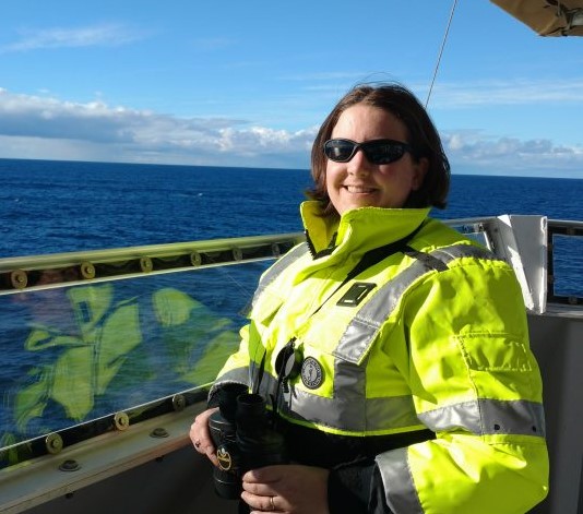
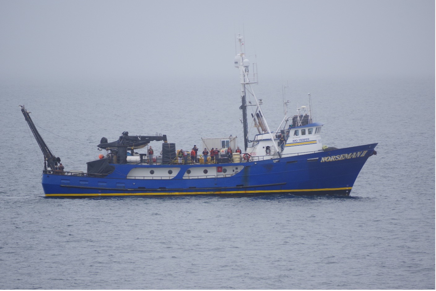
Clara Bird, PhD Candidate, OSU Department of Fisheries, Wildlife, and Conservation Sciences, Geospatial Ecology of Marine Megafauna Lab

As you may remember, last year’s field season was a remarkable summer for our team. We were pleasantly surprised to find an increased number of whales in our study area compared to previous years and were even more excited that many of them were old friends. As we started this field season, we were all curious to know if this year would be a repeat. And it’s my pleasure to report that this season was even better!

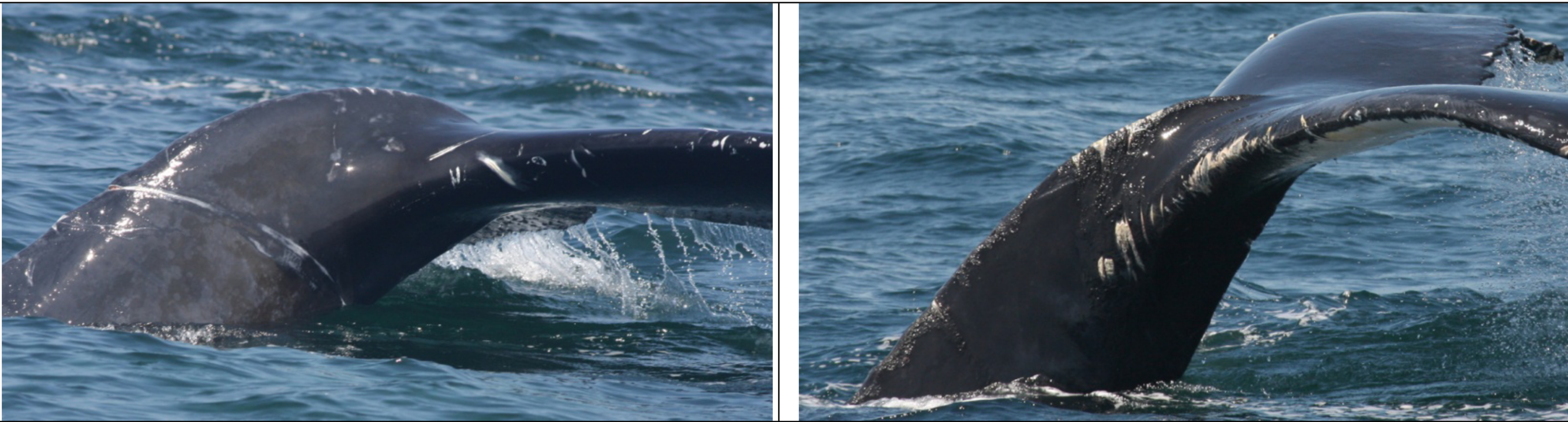
We started the season with an exciting day (6 known whales! see Lisa’s blog) and the excitement (and whales) just kept coming. This season we saw 71 individual whales across 215 sightings! Of those 71, 44 were whales we saw last year, and 10 were new to our catalog, meaning that we saw 17 whales this season that we had not seen in at least two years! There is something extra special about seeing a whale we have not seen in a while because it means that they are still alive, and the sighting gives us valuable data to continue studying health and survival. Another cool note is that 7 of our 12 new whales from last year came back this year, indicating recruitment to our study region.

Included in that group of 7 whales are the two calves from last year! Again, indicating good recruitment of new whales to our study area. We saw both Lunita and Manta (previously nick-named ‘Roly-poly’) throughout this season and we were always happy to see them back in our area and feeding on their own.

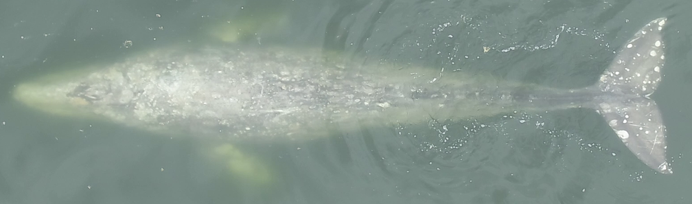
We had an especially remarkable encounter with Lunita at the end of this season when we found this whale surface feeding on porcelain crab larvae (video 1)! This is a behavior that we rarely observe, and we’ve never seen a juvenile whale use this behavior before, inspiring questions around how Lunita knew how to perform this behavior.

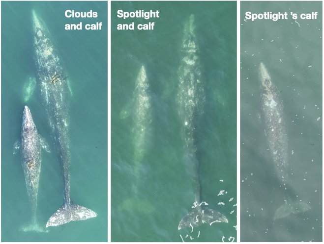
Not only did we resight our one-year-old friends, but we found two new calves born to well-known mature females (Clouds and Spotlight). We had previously documented Clouds with a calf (Cheetah) in 2016 so it was exciting to see her with a new calf and to meet Cheetah’s sibling! Cheetah has become one of our regulars so we’re curious to see if this new calf joins the regular crew as well. We’re also hoping that Spotlight’s calf will stick around; and we’re optimistic since we observed it feeding alone later in the season.

Collage of new calves from 2023! Left: Clouds and her calf, Center: Spotlight and her calf, Right: Spotlight’s calf independently foraging

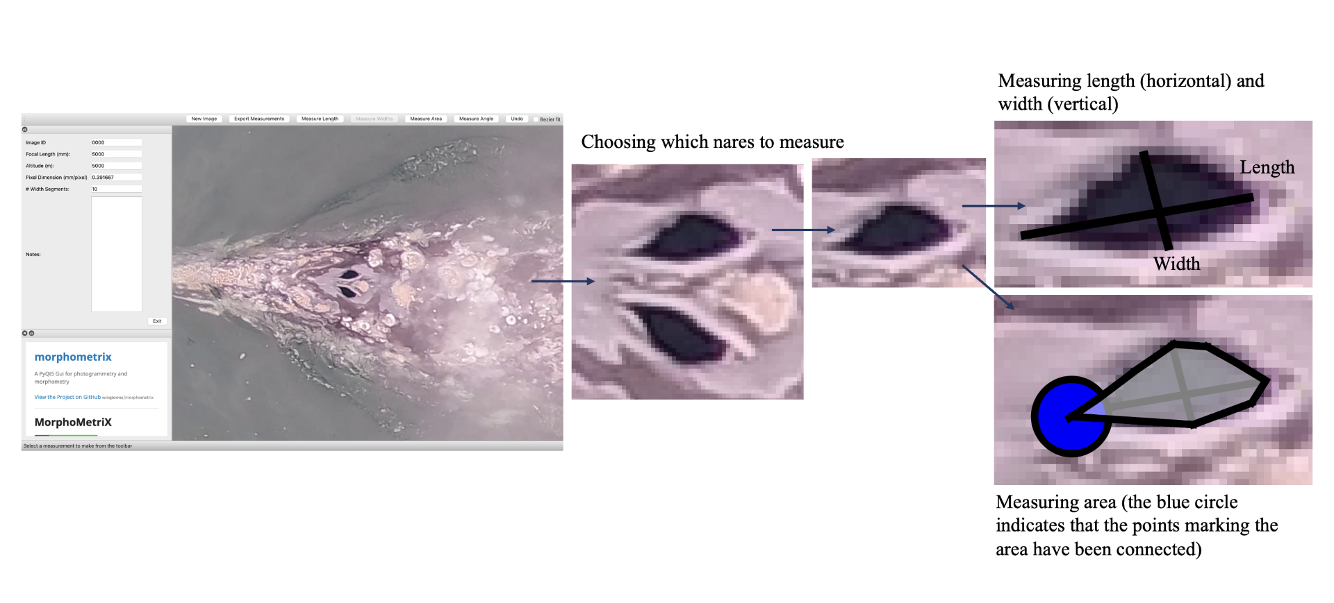
Of course, 71 whales means heaps of data! We spent 226 hours on the water, conducted 132 drone flights (a record!), and collected 61 fecal samples! Those 132 flights were over 64 individual whales, with Casper and Pacman tying for “best whale to fly over” with 10 flights each. We collected 61 fecal samples from 26 individual whales with a three-way tie for “best pooper” between Hummingbird, Scarlett, and Zorro with 6 fecal samples each. And we continued to collect valuable prey and habitat data through 80 GoPro drops and 79 zooplankton net tows.

Above: (left) drone image of the team on our boat next to Pacman, (right) KC piloting the drone. Below: the team celebrating good fecal samples!

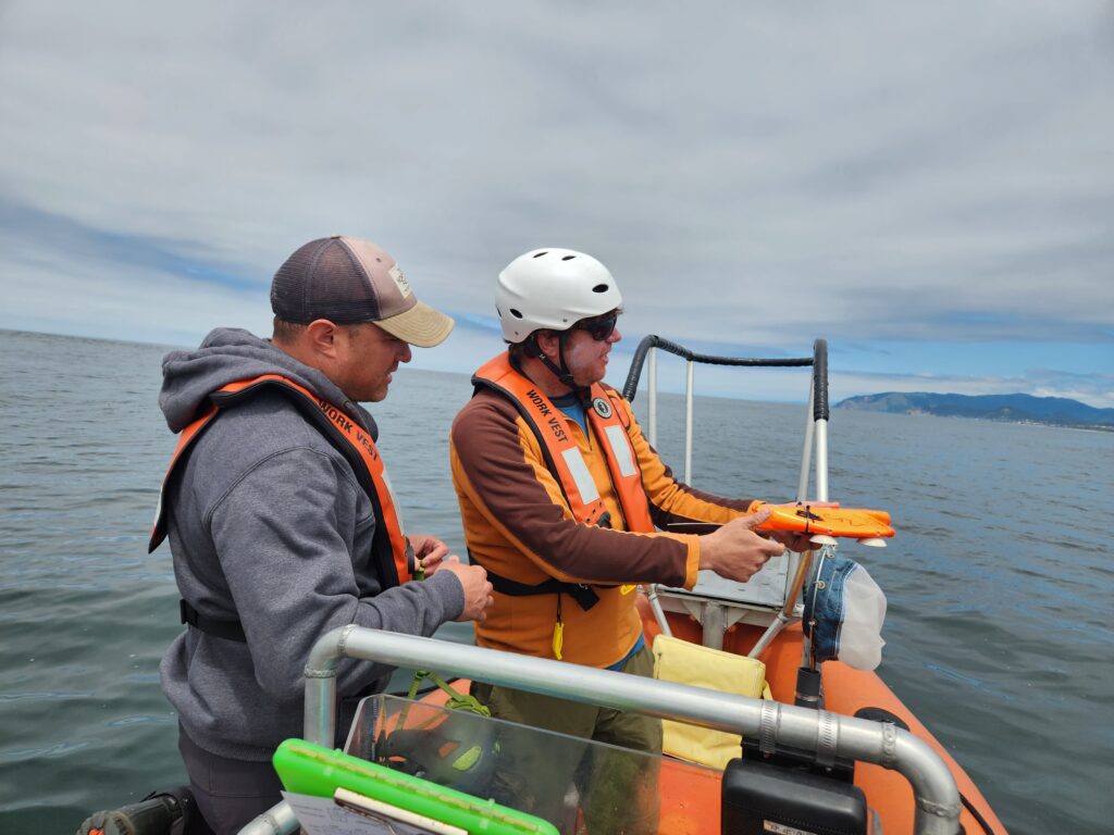
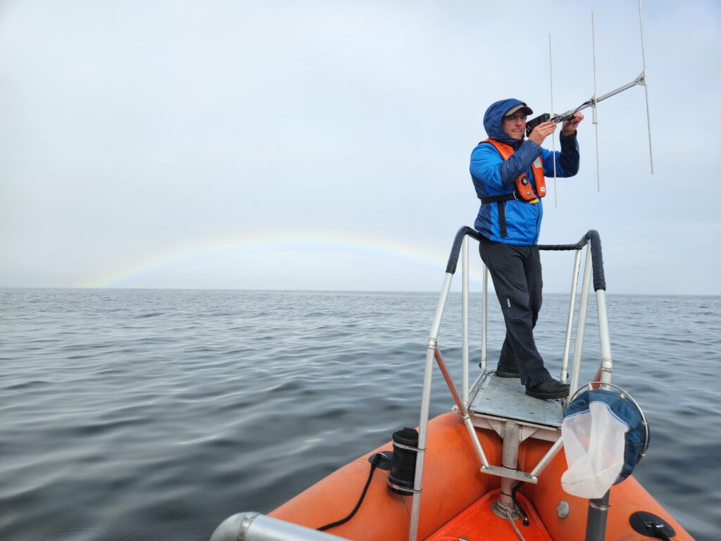
And if you were about to ask, “but what about tagging?!”, fear not! We continued our suction cup tagging effort with a successful window in July where we were joined by collaborators John Calambokidis from Cascadia Research Collective and Dave Cade from Hopkins Marine Station and deployed four suction-cup tags.

The team during our tagging effort this season.

It’s hard to believe all the work we’ve accomplished in the past five months, and I continue to be honored and proud to be on this incredible team. But as this season has come to a close, I have found myself reflecting on something else. Learning. Over the past several years we have learned so much about not only these whales in our study system but about how to conduct field work. And while learning is continuous, this season in particular has felt like an exciting time for both. In the past year our group has published work showing that we can detect pregnancy in gray whales using fecal samples and drone imagery (Fernandez Ajó et al., 2023), that PCFG gray whales are shorter and smaller than ENP whales (Bierlich et al., 2023), and that gray whales are consuming high levels of microplastics (Torres et al., 2023). We also have several manuscripts in review focused on our behavior work from drones and tags. While this information does not directly affect our field work, it does mean that while we’re observing these whales live, we better understand what we’re observing and we can come up with more specific, in-depth questions based on this foundation of knowledge that we’re building. I have enjoyed seeing our questions evolve each year based on our increasing knowledge and I know that our collaborative, inquisitive chats on the boat will only continue inspiring more exciting research.

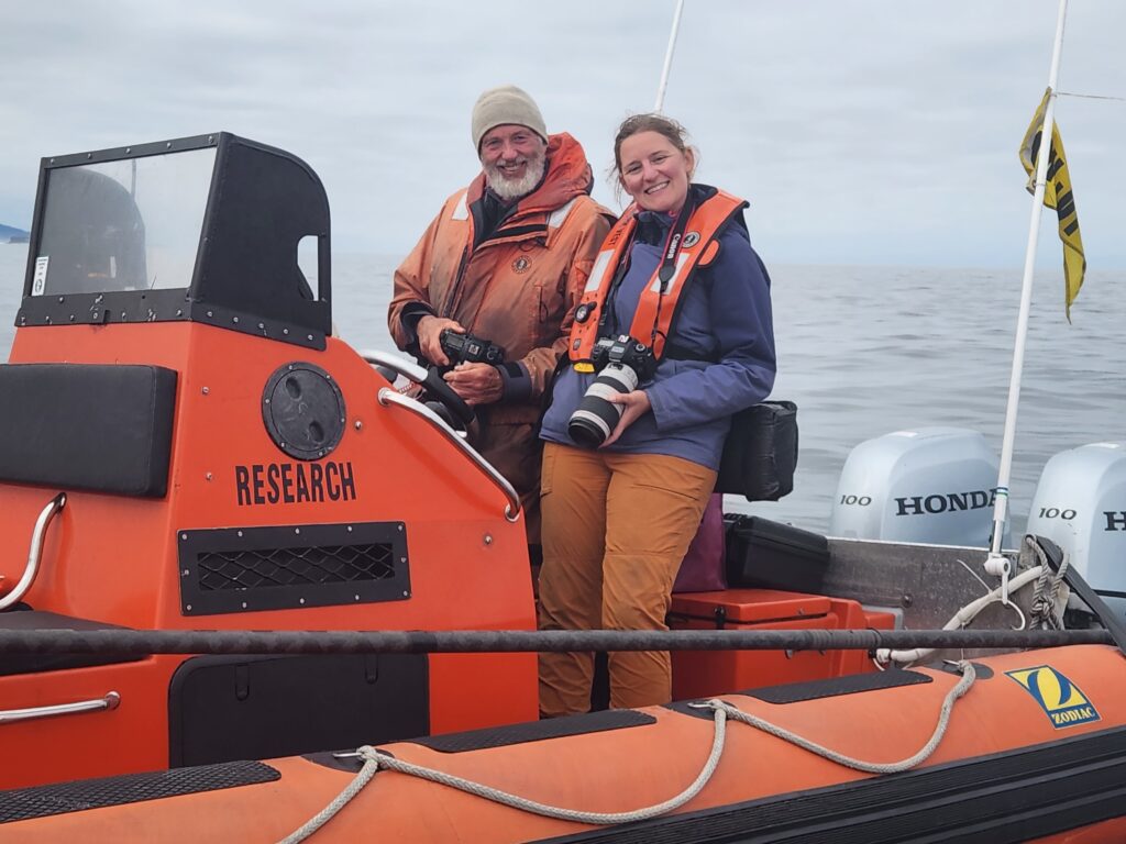
On top of our gray whale knowledge, we have also learned so much about field work. When I think back to the early days compared to now, there is a stark difference in our knowledge and our confidence. We do a lot on our little boat! And so many steps that we once relied on written lists to remember to do are now just engrained in our minds and bodies. From loading the boat, to setting up at the dock, to the go pro drops, fecal collections, drone operations, photo taking, and photo ID, our team has become quite the well-oiled machine. We were also given the opportunity to reflect on everything we’ve learned over the past years when it was our turn to train our new team member, Nat! Nat is a new PhD student in the GEMM lab who is joining team GRANITE. Teaching her all the ins and outs of our fieldwork really emphasized how much we ourselves have learned.

On a personal note, this was my third season as a drone pilot, and honestly, I was pleasantly surprised by my experience this season. Since I started piloting, I have experienced pretty intense nerves every time I’ve flown the drone. From stress dreams, to mild nausea, and an elevated heart rate, flying the drone was something that I didn’t necessarily look forward to. Don’t get me wrong – it’s incredibly valuable data and a privilege to watch the whales from a bird’s eye view in real time. But the responsibility of collecting good data, while keeping the drone and my team members safe was something that I felt viscerally. And while I gained confidence with every flight, the nerves were still as present as ever and I was starting to accept that I would never be totally comfortable as a pilot. Until this season, when the nerves finally cleared, and piloting became as innate as all the other field work components. While there are still some stressful moments, the nerves don’t come roaring back. I have finally gone through enough stressful situations to not be fazed by new ones. And while I am fully aware that this is just how learning works, I write this reflection as a reminder to myself and anyone going through the process of learning any new skill to push through that fear. Remember there can be a disconnect between the time when you know how to do something well, or well-enough, and the time when you feel comfortable doing it. I am just as proud of myself for persevering as I am of the team for collecting so much incredible data. And as I look ahead to my next scary challenge (finishing my PhD!), this is a feeling that I am trying to hold on to.

Stay tuned for updates from team GRANITE!

Did you enjoy this blog? Want to learn more about marine life, research, and conservation? Subscribe to our blog and get a weekly alert when we make a new post! Just add your name into the subscribe box below!

References

Bierlich, K. C., Kane, A., Hildebrand, L., Bird, C. N., Fernandez Ajo, A., Stewart, J. D., Hewitt, J., Hildebrand, I., Sumich, J., & Torres, L. G. (2023). Downsized: Gray whales using an alternative foraging ground have smaller morphology. Biology Letters, 19(8), 20230043. https://doi.org/10.1098/rsbl.2023.0043

Fernandez Ajó, A., Pirotta, E., Bierlich, K. C., Hildebrand, L., Bird, C. N., Hunt, K. E., Buck, C. L., New, L., Dillon, D., & Torres, L. G. (2023). Assessment of a non-invasive approach to pregnancy diagnosis in gray whales through drone-based photogrammetry and faecal hormone analysis. Royal Society Open Science, 10(7), 230452. https://doi.org/10.1098/rsos.230452

Torres, L. G., Brander, S. M., Parker, J. I., Bloom, E. M., Norman, R., Van Brocklin, J. E., Lasdin, K. S., & Hildebrand, L. (2023). Zoop to poop: Assessment of microparticle loads in gray whale zooplankton prey and fecal matter reveal high daily consumption rates. Frontiers in Marine Science, 10. https://www.frontiersin.org/articles/10.3389/fmars.2023.1201078

Cruising through space and time – a GEMM Lab’s journey in the Northern California Current

By Solène Derville, Postdoc, OSU Department of Fisheries, Wildlife, and Conservation Sciences, Geospatial Ecology of Marine Megafauna Lab

Last month I had the privilege to participate in the 2023 September Northern California Current (NCC) cruise onboard the NOAA RV Bell M. Shimada. These cruises are part of a long-term NOAA/NWFSC effort to study the NCC ecosystem and they have been taking place every February, May, and September since 2002. Thanks to a collaboration with NOAA (and more specifically the NCC cruise chief scientist Jennifer Fisher), the GEMM Lab has been able to put marine mammal observers on these cruises since 2018.

As a postdoc working on the OPAL project, I have been the main person in charge of processing and analyzing the cetacean data collected across the 10 (now 11!) cruises that the GEMM lab participated in. These data have played a paramount role in improving our understanding of rorqual whale (e.g., blue, humpback, fin) distribution and habitat use off the coast of Oregon (Derville et al., 2022) and assessing the resulting risk of entanglement in fishing gear that they face while migrating and feeding in our waters (Derville et al., 2023). But while I have been very involved in the data analysis side of things, up to now I had never been able to contribute to data collection for this project. First, I was working remotely at the height of the COVID pandemic and second, because the NCC cruises are onboard a NOAA vessel, they have strict limitations on non-US citizens participation. So, you can imagine how excited I was (as a French citizen) to finally set foot on the famous Bell M. Shimada that I had heard so many stories about!

The NCC cruises illustrate how valuable long-term ecosystem monitoring is. Station after station, miles surveyed after miles surveyed, little by little, we learn about the complex ecological relationships and changing patterns that shape life in the ocean. The data, the experience, and the memories accumulated over the years are a true legacy that I have felt very proud to be part of. Finally, being on this ship, I felt like I was walking in the path of so many of my friends who had held those same binoculars before. Florence Sullivan, who pioneered the GEMM Lab’s NCC cruise observer effort in the harsh winter weather of February 2018. Alexa Kownacki (May 2018, May 2019), whose detailed field notes I read years later with emotion and appreciation as they helped me figure out how the Seebird software used to collect data back then (and abandoned since!). Dawn Barlow (Sep 2018, Sep 2019, Sep 2020, May 2021, May 2022), our master observer who is said to be able to detect a whale’s blow 10 miles away in a 10-foot swell and Beaufort sea state 6, all while sipping an Affogato coffee. Clara Bird (Sep 2020, May 2022), who abandoned her beloved nearshore gray whales (twice!) to sail all the way to the NH-200 station (200 nautical miles from land!). Rachel Kaplan (May 2021, May 2022, Sep 2022), our jack of all trades who concurrently studies krill and whales, and by doing so probably broke the record of numbers of times running up and down between the flying bridge and the echosounder screen room down below. Renee Albertson (Sep 2022), a Marine Mammal Institute research associate who shared observations with Rachel until the cruise was cut short by an engine issue that led them to the docks of Seattle. And finally, Craig Hayslip (May 2023), who swapped his usual observer work on the United States Coast Guard’s helicopters as part of the OPAL project for two weeks onboard the Shimada.

What a team!

From left to right and top to bottom: Florence; Alexa; Dawn; Clara; Renee, Rachel and the rest of the science team including Jennifer Fisher and Anna Bolm; Craig; Rachel; and I!

The 11^th NCC cruise with GEMM Lab observers onboard was equal to its predecessors as it provided a perfect combination of camaraderie, natural beauty, Pacific Northwest weather, and unexpected change of plans. After being delayed by one day, we discovered that a big storm system was coming upon us and would have us retreat to Yaquina Bay in Newport for 4 days! Overall, I spent 5 days surveying for marine mammals from the flying bridge, in conditions that went from a beautiful sunny Friday on September 22^nd to an impressive Beaufort sea state 7 on the 29^th. This experience was the king of weather in which it became particularly cool to be on a ship as big as the Shimada (63 m, 208 feet long!) that can withstand swell and wind better than any ship I had worked on before.

Overall, I observed 36 groups of cetaceans, including seven different species of dolphins and whales: one sperm whale, a possible Sei whale, several fin whales, blue whales, humpback whales, and pods of Pacific white-sided dolphins, Dall’s porpoises and common dolphins. Among the highlights of this cruise was the observation of several blue whales and humpback whales that seemed to be feeding on the western slope of the Heceta bank. My personal favorite memory was also to observe common dolphins -a species that despite its name is not that common (at least not in the nearshore environment) and that I had never seen before in my life! How magnificent and graceful they were… and how lucky was I to be part of this voyage.

From left to right, top to bottom: a CTD deployment from the Bell M. Shimada; a whale’s dinner? Krill collected with a bongo net during a previous cruise; a very distant yet unmistakable sperm whale dorsal knob; a group of common dolphins; a marine mammal observer’s work tools; a blue whale surfacing at dusk.

More NCC cruise stories…

Surprises at Sea

Yonder Whales and Nearby Prey: A New Look at a Familiar System

Roger that, we are currently enamored

Marine mammals of the Northern California Current, 2020 edition

Surveying for marine mammals in the Northern California Current

Marine Mammal Observing: Standardization is key

Albatrosses at sunrise, dolphins at sunset: Northern California Current cruise

The Recipe for a “Perfect” Marine Mammal and Seabird Cruise

Living the Dream – life as a marine mammal observer

References

Derville, S., Barlow, D. R., Hayslip, C. E., & Torres, L. G. (2022). Seasonal, Annual, and Decadal Distribution of Three Rorqual Whale Species Relative to Dynamic Ocean Conditions Off Oregon, USA. Frontiers in Marine Science, 9, 868566. https://doi.org/10.3389/fmars.2022.868566

Derville, S., Buell, T. V, Corbett, K. C., Hayslip, C., & Torres, L. G. (2023). Exposure of whales to entanglement risk in Dungeness crab fishing gear in Oregon, USA, reveals distinctive spatio-temporal and climatic patterns. Biological Conservation, 109989. https://doi.org/10.1016/j.biocon.2023.109989

Fantastic beasts and how to measure them!

Sagar Karki, Master’s student in the Computer Science Department at Oregon State University

What beasts? Good question! We are talking about gray whales in this article but honestly we can tweak the system discussed in this blog a little and make it usable for other marine animals too.

Understanding the morphology, such as body area and length, of wild animals and populations can provide important information on animal behavior and health (check out postdoc Dr. KC Bierlich’s post on this topic). Since 2015, the GEMM Lab has been flying drones over whales to collect aerial imagery to allow for photogrammetric measurements to gain this important morphological data. This photogrammetry data has shed light on multiple important aspects of gray whale morphology, including the facts that the whales feeding off Oregon are skinnier [1] and shorter [2] than the gray whales that feed in the Arctic region. But, these surprising conclusions overshadow the immense, time-consuming labor that takes place behind the scenes to move from aerial images to accurate measurements.

To give you a sense of this laborious process, here is a quick run through of the methods: First the 10 to 15 minute videos must be carefully watched to select the perfect frames of a whale (flat and straight at the surface) for measurement. The selected frames from the drone imagery are then imported into MorphoMetriX, which is a custom software developed for photogrammetry measurement [1]. MorphoMetriX is an interactive application that allows an analyst to manually measure the length by clicking points along the centerline of the whale’s body. Based on this line, the whale is divided into a set of sections perpendicular to the centerline, these are used to then measure widths along the body. The analyst then clicks border points at the edge of the whale’s body to delineate the widths following the whale’s body curve. MorphoMetriX then generates a file containing the lengths and widths of the whale in pixels for each measured image. The length and widths of whales are converted from pixels to metric units using a software called CollatriX [4] and this software also calculates metrics of body condition from the length and width measurements.

While MorphoMetriX [3] and CollatriX [4] are both excellent platforms to facilitate these photogrammetry measurements, each measurement takes time, a keen eye, and attention to detail. Plus, if you mess up one step, such as an incorrect length or width measurement, you have to start from the first step. This process is a bottleneck in the process of obtaining important morphology data on animals. Can we speed this process up and still obtain reliable data?

What if we can apply automation using computer vision to extract the frames we need and automatically obtain measurements that are as accurate as humans can obtain? Sounds pretty nice, huh? This is where I come into the picture. I am a Master’s student in the Computer Science Department at OSU, so I lack a solid background in marine science, but bring to the table my skills as a computer programmer. For my master’s project, I have been working in the GEMM Lab for the past year to develop automated methods to obtain accurate photogrammetry measurements of whales.

We are not the first group to attempt to use computers and AI to speed up and improve the identification and detection of whales and dolphins in imagery. Researchers have used deep learning networks to speed up the time-intensive and precise process of photo-identification of individual whales and dolphins [5], allowing us to more quickly determine animal location, movements and abundance. Millions of satellite images of the earth’s surface are collected daily and scientists are attempting to utilize these images to benefit marine life by studying patterns of species occurrence, including detection of gray whales in satellite images using deep learning [6]. There has also been success using computer vision to identify whale species and segment out the body area of the whales from drone imagery [7]. This process involves extracting segmentation masks of the whale’s body followed by length extraction from the mask. All this previous research shows promise for the application of computer vision and AI to assist with animal research and conservation. As discussed earlier, the automation of image extraction and photogrammetric measurement from drone videos will help researchers collect vital data more quickly so that decisions that impact the health of whales can be more responsive and effective.For instance, photogrammetry data extracted from drone images can diagnose pregnancy of the whales [8], thus automation of this information could speed up our ability to understand population trends.

Computer vision and natural language processing fields are growing exponentially. There are new foundation models like ChatGPT that can do most of the natural language understanding and processing tasks. Foundational models are also emerging for computer vision tasks, such as “the segment anything model” from Meta. Using these foundation models along with other existing research work in computer vision, we have developed and deployed a system that automates the manual and computational tasks of MorphoMetriX and CollatriX systems.

This system is currently in its testing and monitoring phase, but we are rapidly moving toward a publication to disseminate all the tools developed, so stay tuned for the research paper that will explain in detail the methodologies followed on data processing, model training and test results. The following images give a sneak peak of results. Each image illustrates a frame from a drone video that was identified and extracted through automation, followed by another automation process that identified important points along the whale’s body and curvature. The user interface of the system aims to make the user experience intuitive and easy to follow. The deployment is carefully designed to run on different hardwares, with easy monitoring and update options using the latest open source frameworks. The user has to do just two things. First, select the videos for analysis. The system then generates potential frames for photogrammetric analysis (you don’t need to watch 15 mins of drone footage!). Second, the user selects the frame of choice for photogrammetric analysis and waits for the system to give you measurements. Simple! Our goal is for these softwares to be a massive time-saver while still providing vital, accurate body measurements to the researchers in record time. Furthermore, an advantage of this approach is that researchers can follow the methods in our to-be-soon-published research paper to make a few adjustments enabling the software to measure other marine species, thus expanding the impact of this work to many other life forms.

A sneak peek of the results. Each image illustrates a frame from a drone video that was identified and extracted through automation, followed by another automation process that identified important points along the whale’s body and curvature.

Did you enjoy this blog? Want to learn more about marine life, research, and conservation? Subscribe to our blog and get a weekly message when we post a new blog. Just add your name and email into the subscribe box below.

References

Torres LG, Bird CN, Rodríguez-González F, Christiansen F, Bejder L, Lemos L, Urban R J, Swartz S, Willoughby A, Hewitt J, Bierlich K (2022) Range-Wide Comparison of Gray Whale Body Condition Reveals Contrasting Sub-Population Health Characteristics and Vulnerability to Environmental Change. Front Mar Sci 910.3389/fmars.2022.867258

Bierlich KC, Kane A, Hildebrand L, Bird CN, Fernandez Ajo A, Stewart JD, Hewitt J, Hildebrand I, Sumich J, Torres LG (2023) Downsized: gray whales using an alternative foraging ground have smaller morphology. Biol Letters 19:20230043 doi:10.1098/rsbl.2023.0043

Torres et al., (2020). MorphoMetriX: a photogrammetric measurement GUI for morphometric analysis of megafauna. Journal of Open Source Software, 5(45), 1825, https://doi.org/10.21105/joss.01825

Bird et al., (2020). CollatriX: A GUI to collate MorphoMetriX outputs. Journal of Open Source Software, 5(51), 2328, https://doi.org/10.21105/joss.02328

Patton, P. T., Cheeseman, T., Abe, K., Yamaguchi, T., Reade, W., Southerland, K., Howard, A., Oleson, E. M., Allen, J. B., Ashe, E., Athayde, A., Baird, R. W., Basran, C., Cabrera, E., Calambokidis, J., Cardoso, J., Carroll, E. L., Cesario, A., Cheney, B. J. … Bejder, L. (2023). A deep learning approach to photo–identification demonstrates high performance on two dozen cetacean species. Methods in Ecology and Evolution, 00, 1–15. https://doi.org/10.1111/2041-210X.14167

Green, K.M., Virdee, M.K., Cubaynes, H.C., Aviles-Rivero, A.I., Fretwell, P.T., Gray, P.C., Johnston, D.W., Schönlieb, C.-B., Torres, L.G. and Jackson, J.A. (2023), Gray whale detection in satellite imagery using deep learning. Remote Sens Ecol Conserv. https://doi.org/10.1002/rse2.352

Gray, PC, Bierlich, KC, Mantell, SA, Friedlaender, AS, Goldbogen, JA, Johnston, DW. Drones and convolutional neural networks facilitate automated and accurate cetacean species identification and photogrammetry. Methods Ecol Evol. 2019; 10: 1490–1500. https://doi.org/10.1111/2041-210X.13246

Fernandez Ajó A, Pirotta E, Bierlich KC, Hildebrand L, Bird CN, Hunt KE, Buck CL, New L, Dillon D, Torres LG (2023) Assessment of a non-invasive approach to pregnancy diagnosis in gray whales through drone-based photogrammetry and faecal hormone analysis. Royal Society Open Science 10:230452

Familiar flukes and flanks: The 9th GRANITE field season is underway

By Lisa Hildebrand, PhD student, OSU Department of Fisheries, Wildlife, & Conservation Sciences, Geospatial Ecology of Marine Megafauna Lab

The winds are consistently (and sometimes aggressively) blowing from the north here on the Oregon coast, which can only mean one thing – summer has arrived! Since mid-May, the GRANITE (Gray whale Response to Ambient Noise Informed by Technology and Ecology) team has been looking for good weather windows to survey for gray whales and we have managed to get five great field work days already. In today’s blog post, I am going to share what (and who) we have seen so far.

On our first day of the field season, PI Leigh Torres, postdoc KC Bierlich and myself, were joined by a special guest: Dr. Andy Read. Andy is the director of the Duke University Marine Lab, where he also runs his own lab, which focuses on conservation biology and ecology of marine vertebrates. Andy was visiting the Hatfield Marine Science Center as part of the Lavern Weber Visiting Scientist program and was hosted here by Leigh. For those of you that do not know, Andy was Leigh’s graduate school advisor at Duke where she completed her Master’s and doctoral degrees. It felt very special to have Andy on board our RHIB Ruby for the day and to introduce him to some friends of ours. The first whale we encountered that day was “Pacman”. While we are always excited to re-sight an individual that we know, this sighting was especially mind-blowing given the fact that Leigh had “just” seen Pacman approximately two months earlier in Guerrero Negro, one of the gray whale breeding lagoons in Mexico (read this blog about Leigh and Clara’s pilot project there). Aside from Pacman, we saw five other individuals, all of which we had seen during last year’s field season.

*The first day of field work for the 2023 GRANITE field season! From left to right: Leigh Torres, Lisa Hildebrand, Andy Read, and KC Bierlich. Source: L. Torres.*

Since that first day on the water, we have conducted field work on four additional days and so far, we have only encountered known individuals in our catalog. This fact is exciting because it highlights the strong site fidelity that Pacific Coast Feeding Group (PCFG) gray whales have to areas within their feeding range. In fact, I am examining the residency and space use of each individual whale we have observed in our GRANITE study for one of my PhD chapters to better understand the level of fidelity individuals have to the central Oregon coast. Furthermore, this site fidelity underpins the unique, replicate data set on individual gray whale health and ecology that the GRANITE project has been able to progressively build over the years. So far during this field season in 2023, we have seen 13 unique individuals, flown the drone over 10 of them and collected four fecal samples from two, which represent critical data points from early on in the feeding season.

Our sightings this year have not only highlighted the high site fidelity of whales to our study area but have also demonstrated the potential for internal recruitment of calves born to “PCFG mothers” into the PCFG. Recruitment to a population can occur in two ways: externally (individuals immigrate into a population from another population) or internally (calves born to females that are part of the population return to, or stay, within their mothers’ population). Three of the whales we have seen so far this year are documented calves from females that are known to consistently use the PCFG range, including our central Oregon coast study area. In fact, we documented one of these calves, “Lunita”, just last year with her mother (see Clara’s recap of the 2022 field season blog for more about Lunita). The average calf survival estimate between 1997-2017 for the PCFG was 0.55 (Calambokidis et al. 2019), though it varied annually and widely (range: 0.34-0.94). Considering that there have been years with calf survival estimates as low as ~30%, it is therefore all the more exciting when we re-sight a documented calf, alive and well!

*“Lunita”, an example of successful internal recruitment*

We have also been collecting data on the habitat and prey in our study system by deploying our paired GoPro/RBR sensor system. We use the GoPro to monitor the benthic substrate type and relative prey densities in areas where whales are feeding. The RBR sensor collects high-frequency, in-situ dissolved oxygen and temperature data, enabling us to relate environmental metrics to relative prey measurements. Furthermore, we also collect zooplankton samples with a net to assess prey community and quality. On our five field work days this year, we have predominantly collected mysid shrimp, including gravid (a.k.a. pregnant) individuals, however we have also caught some Dungeness and porcelain crab larvae. The GEMM Lab is also continuing our collaboration with Dr. Susanne Brander’s lab at OSU and her PhD student Lauren Kashiwabara, who plan on conducting microplastic lab experiments on wild-caught mysid shrimp. Their plan is to investigate the growth rates of mysid shrimp under different temperature, dissolved oxygen, and microplastic load conditions. However, before they can begin their experiments, they need to successfully culture the mysids in the lab, which is why we collect samples for them to use as their ‘starter culture’. Stay tuned to hear more about this project as it develops!

So, all in all, it has been an incredibly successful start to our field season, marked by the return of many familiar flukes and flanks! We are excited to continue collecting rock solid GRANITE data this summer to increase our efforts to understand gray whale ecology and physiology.

References

Calambokidis, J., Laake, J., and Perez, A. (2019). Updated analyses of abundance and population structure of seasonal gray whales in the Pacific Northwest, 1996-2017. IWC, SC/A17/GW/05 for the Workshop on the Status of North Pacific Gray Whales. La Jolla: IWC.

Title: “Blown away”: measuring the blowholes of whales from drones

By Annie Doron, Undergraduate Intern, Oregon State University, GEMM Laboratory

Hey up! My name is Annie Doron, and I am an undergraduate Environmental Science student from the University of Sheffield (UK) on my study year abroad. One of my main motivations for undertaking this year abroad was to gain experience working in a marine megafauna lab. Whales in particular have always captivated my interest, and I have been lucky enough to observe humpback whales in Iceland and The Azores, and even encountered one whilst diving in Australia! For the past 10 months, I have had the unique opportunity to work in the GEMM Lab analyzing Pacific Coast Feeding Group (PCFG) gray whales off the Oregon Coast (Figure 1). I must admit, it has been simply wonderful!

Figure 1. Aerial image of a PCFG gray whale off the Oregon Coast.

How did I end up getting involved with the GEMM Lab? I was first accepted into Scarlett Arbuckle’s research-based class in fall term 2022, which is centered around partnering with a mentor for a research project. Having explored the various fields of research at HMSC, I contacted Leigh Torres with interest in getting involved in the GEMM Lab and to establish a research project suitable for a totally inexperienced, international, undergraduate student. Thankfully, Leigh forwarded my email to KC Bierlich who offered to be my mentor for the class, and the rest is history! I first began analyzing drone imagery to measure length and body condition of PCFG gray whales, which provided an opportunity to get involved with the lab and gain experience using the photogrammetry software MorphoMetriX (Torres & Bierlich, 2020) (see KC’s blog), which is used to make morphometric measurements of whales. Viewing drone imagery of whales sparked my interest in how they use their blowholes (otherwise called ‘nares’) to replenish their oxygen stores; this led to us establishing a research project for the class where we tested if we could use MorphoMetriX to measure blowholes from drone imagery.

Extending this project into winter and spring terms (via research credits) has enabled me to continue working with Leigh and KC, as well as to collaborate with Clara Bird and Jim Sumich. Thanks to KC, who has patiently guided me through the ins and outs of working on a research project, I now feel more confident handling and manipulating large datasets, analyzing drone footage (i.e., differentiating between behavioral states, recording breathing sequences, detecting when a whale is exhaling vs inhaling, etc.), and speaking in public (although I still get pretty bad stage fright, but I think that is a typical conundrum undergrads face). Whatsmore, applying R – a programming language used for statistical analysis and data visualization, which I have been trying to wrap my head around for years – to my own dataset has helped me greatly enhance my skills using it.

So, what exciting things have we been working on this year? Given that we often cannot simply study a whale from inside a laboratory – due to size-related logistical implications – we must use proxies (i.e., a variable that is representative of an immeasurable variable). Since cetaceans must return to the surface to offload carbon dioxide and replenish their oxygen stores, measuring their breath frequency and magnitude is one way to study a whale’s oxygen consumption, in turn offering insight into its energy expenditure (Williams, 1999). Blowholes are one proxy we can use to study breath magnitude. Blowholes can be utilized in this way by measuring inhalation duration (the amount of time a whale is inhaling, which is based on a calculation developed by Jim Sumich) and blowhole area (the total area of a blowhole) to gauge variations in tidal volume (the amount of air flowing in and out of the lungs).

Measuring inhalation duration and blowhole area is important because a larger blowhole area (i.e., one that is more dilated) and a longer inhalation duration is indicative of higher oxygen intake, which can infer stress. For example, in this population, higher stress levels are associated with increased vessel traffic (Lemos et al., 2022), and skinnier whales have higher stress levels compared to chubby, healthy whales (Lemos, Olsen, et al., 2022). Hence, measuring the variation around blowholes could be utilized to predict challenges whales face from climate change and anthropogenic disturbance, including fishing (Scordino et al., 2017) and whale watching industry threats (Sullivan & Torres, 2018) (see Clara’s blog), as well as to inform effective management strategies. Furthermore, measuring the variables inhalation duration and blowhole area could help to identify whether whales are taking larger breaths associated with certain ‘gross behavior states’, otherwise known as ‘primary states’, which include: travel, forage, rest, social (Torres et al., 2018). This could enable us to assess the energetic costs of different foraging tactics (i.e., head standing, side-swimming, and bubble blasting (Torres et al., 2018), as well as consequences of disturbance events, on an individual and population health perspective.

Inhalation duration has been explored in the past by using captive animals. For example, there have been studies on heart rate and breathing of bottlenose dolphins in human care facilities (Blawas et al., 2021; Fahlman et al., 2015). Recently, Nazario et al. (2022) was able to measure inhalation duration and blowhole area using suction-cup video tags. Her study led us to consider if it was possible to measure the parameters and variation around respiration by measuring blowhole area and inhalation duration of PCFGs from drone imagery. We employed MorphoMetriX to study the length, width, and area of a blowhole (Figure 2). Preliminary analyses verified that the areas of the left and right blowholes are very similar (Figure 3); this finding saved us a lot of time because from thereon we only measured either the left or right side. Interestingly, we see some variation in blowhole area within and across individuals (Figure 4). This variation changes within individuals based on primary state. For example, the whales “Glacier”, “Nimbus”, and “Rat” show very little variation whilst traveling but a large amount whilst foraging. Comparatively, “Dice” shows little variation whilst foraging and large variation whilst traveling. Whilst considering cross-individual comparisons, we can see that “Sole”, “Rat”, “Nimbus”, “Heart”, “Glacier”, “Dice”, and “Coal” each exhibit relatively large amounts of variation, yet “Mahalo”, “Luna”, “Harry”, “Hummingbird” and “Batman” exhibit very little. One potential reason for some individuals displaying higher levels of variation than others could be higher levels of exposure to disturbance events that we were unable to measure or evaluate in this study.

Figure 2. How we measured the length, width, and area of a blowhole using MorphoMetriX.

Figure 3. Data driven evidence that the left and the right blowhole areas are very similar.

Figure 4. Variation in blowhole area amongst individual PCFG whales. The hollow circles represent the means, and the color represents the primary state the whale is exhibiting, foraging (purple) vs. traveling (blue), which will be further explored in Clara’s PhD.

Now, we are venturing into June and are at a stage where we (KC, Clara, Jim, Leigh, and I) are preparing to publish a manuscript! What a way to finish such a fantastic year! The transition from a 3-month-long pilot study to a much larger data analysis and eventual preparation for a manuscript has been a monumental learning experience. If anybody had told me a year ago that I would be involved in publishing a body of work – especially one that is so meaningful to me – I would simply not have believed them! We hope this established methodology for measuring blowholes will help other researchers carry out blowhole measurements using drone imagery across different populations and species. Further research is required to explore the differences in inhalation duration and blowhole area between different primary states, specifically across different foraging tactics.

It has been a great privilege working with the GEMM Lab these past months, and I was grateful to be included in their monthly lab meetings, during which members gave updates and we discussed recently published papers. Seeing such an enthusiastic, kind, and empathic group of people working together taught me what working in a supportive lab could look and feel like. In spite of relocating from Corvallis to Bend after my first term, I was happy to be able to continue working remotely for the lab for the remainder of my time (even though I was ~200 miles inland). I thoroughly enjoyed living in Corvallis, highlights of which were scuba diving adventures to the Puget Sound and coastal road trips with friends. The appeal to move arose from Bend’s reputation as an adventure hub – with unlimited opportunities for backcountry ski access – as well as its selection of wildlife ecology courses (with a focus on species specific to central Oregon). I moved into ‘Bunk & Brew’ (Bend’s only hostel, which is more like a big house of friends with occasional hostel guests) on January 1^st after returning from spending Christmas with friends in my old home in Banff, Canada. I have since been enjoying this wonderful multifaceted lifestyle; working remotely in the GEMM Lab, attending in-person classes, working part-time at the hostel, as well as skiing volcanoes (Mount Hood, Middle and South Sister (Figure 5) or climbing at Smith Rock during my days off. Inevitably, I do miss the beautiful Oregon coast, and I will always be grateful for this ideal opportunity and hope this year marks the start of my marine megafauna career!

Figure 5. What I get up to when I’m not studying blowholes! (This was taken at 5am on the long approach to Middle and North Sister. North Sister is the peak featured in the backdrop).

References

Blawas, A. M., Nowacek, D. P., Allen, A. S., Rocho-Levine, J., & Fahlman, A. (2021). Respiratory sinus arrhythmia and submersion bradycardia in bottlenose dolphins (Tursiops truncatus). Journal of Experimental Biology, 224(1), jeb234096. https://doi.org/10.1242/jeb.234096

Fahlman, A., Loring, S. H., Levine, G., Rocho-Levine, J., Austin, T., & Brodsky, M. (2015). Lung mechanics and pulmonary function testing in cetaceans. Journal of Experimental Biology, 218(13), 2030–2038. https://doi.org/10.1242/jeb.119149

Lemos, L. S., Haxel, J. H., Olsen, A., Burnett, J. D., Smith, A., Chandler, T. E., Nieukirk, S. L., Larson, S. E., Hunt, K. E., & Torres, L. G. (2022). Effects of vessel traffic and ocean noise on gray whale stress hormones. Scientific Reports, 12(1), 18580. https://doi.org/10.1038/s41598-022-14510-5

Lemos, L. S., Olsen, A., Smith, A., Burnett, J. D., Chandler, T. E., Larson, S., Hunt, K. E., & Torres, L. G. (2022). Stressed and slim or relaxed and chubby? A simultaneous assessment of gray whale body condition and hormone variability. Marine Mammal Science, 38(2), 801–811. https://doi.org/10.1111/mms.12877

Nazario, E. C., Cade, D. E., Bierlich, K. C., Czapanskiy, M. F., Goldbogen, J. A., Kahane-Rapport, S. R., van der Hoop, J. M., San Luis, M. T., & Friedlaender, A. S. (2022). Baleen whale inhalation variability revealed using animal-borne video tags. PeerJ, 10, e13724. https://doi.org/10.7717/peerj.13724

Scordino, J., Carretta, J., Cottrell, P., Greenman, J., Savage, K., & Scordino, J. (2017). Ship Strikes and Entanglements of Gray Whales in the North Pacific Ocean. Cambridge: International Whaling Commission, 1924–2015.

Sullivan, F. A., & Torres, L. G. (2018). Assessment of vessel disturbance to gray whales to inform sustainable ecotourism: Vessel Disturbance to Whales. The Journal of Wildlife Management, 82(5), 896–905. https://doi.org/10.1002/jwmg.21462

Sumich, J. L. (1994). Oxygen extraction in free-swimming gray whale caves. Marine Mammal Science, 10(2), 226–230. https://doi.org/10.1111/j.1748-7692.1994.tb00266.x

Torres, W., & Bierlich, K. (2020). MorphoMetriX: A photogrammetric measurement GUI for morphometric analysis of megafauna. Journal of Open Source Software, 5(45), 1825. https://doi.org/10.21105/joss.01825

Torres, L. G., Nieukirk, S. L., Lemos, L., & Chandler, T. E. (2018). Drone Up! Quantifying Whale Behavior From a New Perspective Improves Observational Capacity. Frontiers in Marine Science, 5, 319. https://doi.org/10.3389/fmars.2018.00319
Williams, T. M. (1999). The evolution of cost efficient swimming in marine mammals: Limits to energetic optimization. Philosophical Transactions of the Royal Society of London. Series B: Biological Sciences, 354(1380), 193–201. https://doi.org/10.1098/rstb.1999.0371

As waters warm, what are “anomalous conditions” in the face of climate change?

By Dr. Dawn Barlow, Postdoctoral Scholar, OSU Department of Fisheries, Wildlife, and Conservation Sciences, Geospatial Ecology of Marine Megafauna Lab

Recently, I had the opportunity to attend the Effects of Climate Change on the World’s Ocean (ECCWO) conference. This meeting brought together experts from around the world for one week in Bergen, Norway, to gather and share the latest information on how oceans are changing, what is at risk, responses that are underway, and strategies for increasing climate resilience, mitigation, and adaptation. I presented our recent findings from the EMERALD project, which examines gray whale and harbor porpoise distribution in the Northern California Current over the past three decades. Beyond sharing my postdoctoral research widely for the first time and receiving valuable feedback, the ECCWO conference was an incredibly fruitful learning experience. Marine mammals can be notoriously difficult to study, and often the latest methodological approaches or conceptual frameworks take some time to make their way into the marine mammal field. At ECCWO, I was part of discussions at the ground floor of how the scientific community can characterize the impacts of climate change on the ecosystems, species, and communities we study.

One particular theme became increasingly apparent to me throughout the conference: as the oceans warm, what are “anomalous conditions”? There was an interesting dichotomy between presentations focusing on “extreme events,” “no-analog conditions,” or “non-stationary responses,” compared with discussions about the overall trend of increasing temperatures due to climate change. Essentially, the question that kept arising was, what is our frame of reference? When measuring change, how do we define the baseline?

Marine heatwaves have emerged as an increasingly prevalent phenomenon in recent years (see previous GEMM Lab blogs about marine heatwaves here and here). The currently accepted and typically applied definition of a marine heatwave is when water temperatures exceed a seasonal threshold (greater than the 90^th percentile) for a given length of time (five consecutive days or longer) (Hobday et al. 2016). These marine heatwaves can have substantial ecosystem-wide impacts including changes in water column structure, primary production, species composition, distribution, and health, and fisheries management such as closures and quota changes (Cavole et al. 2016, Oliver et al. 2018). Through some of our own previous research, we documented that blue whales in Aotearoa New Zealand shifted their distribution (Barlow et al. 2020) and reduced their reproductive effort (Barlow et al. 2023) in response to marine heatwaves. Concerningly, recent projections anticipate an increase in the frequency, intensity, and duration of marine heatwaves under global climate change (Frölicher et al. 2018, Oliver et al. 2018).

However, as the oceans continue to warm, what baseline do we use to define anomalous events like marine heatwaves? Members of the US National Oceanic and Atmospheric Administration (NOAA) Marine Ecosystem Task Force recently put forward a comment article in Nature, proposing revised definitions for marine heatwaves under climate change, so that coastal communities have the clear information they need to adapt (Amaya et al. 2023). The authors posit that while a “fixed baseline” approach, which compares current conditions to an established period in the past and has been commonly used to-date (Hobday et al. 2016), may be useful in scenarios where a species’ physiological limit is concerned (e.g., coral bleaching), this definition does not incorporate the combined effect of overall warming due to climate change. A “shifting baseline” approach to defining marine heatwaves, in contrast, uses a moving window definition for what is considered “normal” conditions. Therefore, this shifting baseline approach would account for long-term warming, while also calculating anomalous conditions relative to the current state of the system.

*An overview of two different definitions for marine heatwaves, relative to either fixed or shifting baselines. Reproduced from* *Amaya et al. 2023*.

Why bother with these seemingly nuanced definitions and differences in terminology, such as fixed versus shifting baselines for defining marine heatwave events? The impacts of these events can be extreme, and potentially bear substantial consequences to ecosystems, species, and coastal communities that rely on marine resources. With the fixed baseline definition, we may be headed toward perpetual heatwave conditions (i.e., it’s almost always hotter than it used to be), at which point disentangling the overall warming trends from these short-term extremes becomes nearly impossible. What the shifting baseline definition means in practice, however, is that in the future temperatures would need to be substantially higher than the historical average in order to qualify as a marine heatwave, which could obscure public perception from the concerning reality of warming oceans. Yet, the authors of the Nature comment article claim, “If everything is extremely warm all of the time, then the term ‘extreme’ loses its meaning. The public might become desensitized to the real threat of marine heatwaves, potentially leading to inaction or a lack of preparedness.” Therefore, clear messaging surrounding both long-term warming and short-term anomalous conditions are critically important for adaptation and resource allocation in the face of rapid environmental change.

While the findings presented and discussed at an international climate change conference could be considered quite disheartening, I left the ECCWO conference feeling re-invigorated with hope. Crown Prince Haakon of Norway gave the opening plenary and articulated that “We need wise and concerned scientists in our search for truth”. Later in the week, I was a co-convenor of a session that gathered early-career ocean professionals, where we discussed themes such as how we deal with uncertainty in our own climate change-related ocean research, and importantly, how do we communicate our findings effectively. Throughout the meeting, I had formal and informal discussions about methods and analytical techniques, and also about what connects each of us to the work that we do. Interacting with driven and dedicated researchers across a broad range of disciplines and career stages gave me some renewed hope for a future of ocean science and marine conservation that is constructive, collaborative, and impactful.

*Enjoying the ~anomalously~ sunny April weather in Bergen, Norway, during the ECCWO conference.*

Now, as I am diving back in to understanding the impacts of environmental conditions on harbor porpoise and gray whale habitat use patterns through the EMERALD project, I am keeping these themes and takeaways from the ECCWO conference in mind. The EMERALD project draws on a dataset that is about as old as I am, which gives me some tangible perspective on how things have things changed in the Northern California Current during my lifetime. We are grappling with what “anomalous” conditions are in this dynamic upwelling system on our doorstep, whether these anomalies are even always bad, and how conditions continue to change in terms of cyclical oscillations, long-term trends, and short-term events. Stay tuned for what we’ll find, as we continue to disentangle these intertwined patterns of change.

References

Amaya DJ, Jacox MG, Fewings MR, Saba VS, Stuecker MF, Rykaczewski RR, Ross AC, Stock CA, Capotondi A, Petrik CM, Bograd SJ, Alexander MA, Cheng W, Hermann AJ, Kearney KA, Powell BS (2023) Marine heatwaves need clear definitions so coastal communities can adapt. Nature 616:29–32.

Barlow DR, Bernard KS, Escobar-Flores P, Palacios DM, Torres LG (2020) Links in the trophic chain: Modeling functional relationships between in situ oceanography, krill, and blue whale distribution under different oceanographic regimes. Mar Ecol Prog Ser 642:207–225.

Barlow DR, Klinck H, Ponirakis D, Branch TA, Torres LG (2023) Environmental conditions and marine heatwaves influence blue whale foraging and reproductive effort. Ecol Evol 13:e9770.

Cavole LM, Demko AM, Diner RE, Giddings A, Koester I, Pagniello CMLS, Paulsen ML, Ramirez-Valdez A, Schwenck SM, Yen NK, Zill ME, Franks PJS (2016) Biological impacts of the 2013–2015 warm-water anomaly in the northeast Pacific: Winners, losers, and the future. Oceanography 29:273–285.

Frölicher TL, Fischer EM, Gruber N (2018) Marine heatwaves under global warming. Nature 560.

Hobday AJ, Alexander L V., Perkins SE, Smale DA, Straub SC, Oliver ECJ, Benthuysen JA, Burrows MT, Donat MG, Feng M, Holbrook NJ, Moore PJ, Scannell HA, Sen Gupta A, Wernberg T (2016) A hierarchical approach to defining marine heatwaves. Prog Oceanogr.

Oliver ECJ, Donat MG, Burrows MT, Moore PJ, Smale DA, Alexander L V., Benthuysen JA, Feng M, Sen Gupta A, Hobday AJ, Holbrook NJ, Perkins-Kirkpatrick SE, Scannell HA, Straub SC, Wernberg T (2018) Longer and more frequent marine heatwaves over the past century. Nat Commun 9:1–12.

Navigating the Research Rollercoaster

By Amanda Rose Kent, College of Earth Ocean and Atmospheric Sciences, OSU, GEMM Lab/Krill Seeker undergraduate intern

If you asked me five years ago where I’d thought I’d be today, the answer I would give would not reflect where I am now. Back then, I was a customer service representative for a hazardous waste company, and I believed that going to university and participating in research was a straightforward experience. I learned soon after I left that career and began my journey at OSU in 2020 that I wasn’t even remotely aware of the process. I knew that as part of my oceanography degree I would need to become involved in some form of research, but I had no idea where to start.

I started looking through the Oregon State website and I eventually found an outdated flier from 2018 that advertised a lab that studied plankton in Antarctica, and that was when I first reached out to Dr. Kim Bernard. My journey took off from there. As an undergraduate researcher in the URSA Engage program working with Kim and one of her graduate students, Rachel, I conducted a literature review on the ecosystem services provided by two species of krill off the coast of Oregon, including their value to baleen whales. After learning all I could from the literature about krill and how important they were to the ocean, I knew that there was so much more to learn and that this was the topic I wanted to continue to pursue. After I completed the URSA program, I remained a member of Kim’s zooplankton ecology lab.

While continuing to work with Rachel, I was given the opportunity to join the GEMM Lab’s Project HALO for a daylong cruise conducting a whale survey along the Newport Hydrographic Line. I was initially brought on to learn how to use the echosounder to collect krill data but unfortunately, the device had technical difficulties and Rachel and I were no longer needed. We decided to go on the cruise anyway, and I was able to instead learn how to survey for marine mammals (it’s not as easy as it may seem, but still very fun!).

**Figure 1.** Enjoying the point of view from the crow’s nest on the R/V *Pacific Storm*, but also very cold.

Soon, another opportunity arose to apply for a brand-new program called ARC-Learn. This two-year research program focuses on studying the Arctic using publicly available data, and with the support of my mentors, I applied and was accepted. Initially I found that there were no mentors within the program that studied krill, so I found myself becoming immersed in a new topic: harmful algal blooms (HABs). Determined to incorporate krill into this research, I started looking through the literature trying to develop my hypothesis that HABs affected zooplankton in some way. There was evidence to potentially support my hypothesis, but I ended up encountering numerous data gaps in the region I was studying. After months of roadblocks, I eventually started feeling defeated and regretted applying for the program. Rachel was quick to remind me that all experiences are valuable experiences, and that I was still gaining new skills I could use in graduate school or my career.

As my undergraduate degree progressed, I continued supporting Rachel in her graduate research, spending some time during the summer processing krill samples by sorting, sexing, and drying them to crush them into pellets. Our goal was to process them in an instrument called a bomb calorimeter, which is used to quantify the caloric content of prey species and help us better understand the energy flux required for animals higher up the food chain (like whales) and the amount they need to eat. I was only able to do this for a few weeks before heading out on the experience of a lifetime, spending three weeks on a ship traveling around the Bering, Chukchi, and Beaufort Seas with one of my ARC-Learn mentors. It was a great opportunity for me to see the toxic phytoplankton (which can form HABs) I had been studying and learn about methods of sample collection and processing. If I could go back and do it again, I’d go in a heartbeat.

**Figure 2.** Pulling out all of the animal biomass out of the Arctic sediment.

At the beginning of my bachelor’s degree, I had expected to just work with Kim and conduct research within her lab. Instead, I have had opportunities I would never have expected five years ago. I have learned a vast amount from my graduate mentor, Rachel, which has helped influence my trajectory in my degree. I have had the privilege to not only meet giants in the field I’m interested in, but also work with them and learn from them, and to spend three weeks in the Arctic Ocean. The experiences I have had throughout this roller-coaster helped me develop a project idea with new mentors that I eventually hope to pursue in my master’s degree. I wasn’t prepared for the number of adjustments I would make to find new experiences and start new projects, but all the experiences I had were necessary to learn about what I was interested in and what I wanted to pursue. Looking back on it all today, I have zero regrets.

**Figure 3**. A picture of the Norseman II, the ship I was on in the Arctic, taken by the Japanese ship JAMSTEC on a short rendezvous between the Chukchi and Beaufort Seas.

SST, EKE, SSH: Wading Through the Alphabet Soup of Oceanographic Parameters related to Deep-Dwelling Odontocetes

By: Marissa Garcia, PhD Student, Cornell University, Department of Natural Resources and the Environment, K. Lisa Yang Center for Conservation Bioacoustics

Predator-Prey Inference: A Tale as Old as Time

It’s a tale as old as time: where there’s prey, there’ll be predators.

As apex predators, cetaceans act as top-down regulators of ecosystem function. While baleen whales act as “ecosystem engineers,” facilitating nutrient cycling in the ocean (Roman et al., 2014), toothed whales, or “odontocetes,” can impart keystone-level effects — that is, they disproportionately control the marine community’s food-web structure (Valls, Coll, & Christensen, 2015). The menus of prey vary widely by species — ranging from mircronekton to fish to squid – and by extension, vary widely across trophic levels.

So, it naturally follows the old adage: where there’s an abundance of prey, there’ll be an abundance of cetaceans. Yet, creating models that accurately depict this predator-prey relationship is, perhaps unsurprisingly, not as straightforward.

Detecting the ‘Predator’ Half of the Equation

Scientists have successfully documented cetacean presence drawing upon a myriad of methods, each bearing its unique advantages and limitations.

Visual surveys — spanning viewpoints from land, boats, and air — can attain precise spatial data and species ID. However, this data can be constrained by “availability bias” — that is, scientists can only observe cetaceans visible at the surface, not those obscured by the ocean’s depths. Species that spend less time near the surface are more likely to elude the observer’s line of sight, thereby being missed in the data. Consequently, visual surveys have historically undersampled deep-diving species. For instance, since its discovery by western science in 1945, the Hubb’s beaked whale (Mesoplodon carlshubbi) has only been observed alive twice by OSU MMI’s very own Bob Pitman, once in 1994 and another time in 2021.

Scientists have also been increasingly conducting acoustic surveys to document cetacean presence. Acoustic recorders can “hear” each cetacean species at different ranges. Baleen whales, which bellow low-frequency calls, can be heard as far as across ocean basins (Munk et al., 1994). Toothed whales whistle, echolocate, and buzz at frequencies so high they’re considered ultrasonic. But it comes at a trade-off: high-frequency sounds have shorter wavelengths, meaning they are heard across smaller ranges. This high variability, which scientists refer to as “detection range,” translates to not always knowing where the vocalizing cetacean that was recorded is: as such, acoustic data can lack the high-resolution spatial precision often achieved by visual surveys. Nevertheless, acoustic data triumphs in temporal extent, sometimes managing to record continuously at six months at a time. Additionally, animals can elude visual detection in poor weather conditions or if they have a cryptic surface expression, but detected in acoustic surveys (e.g., North Atlantic right whales (Eubalaena glacialis) (Ganley, Brault, & Mayo, 2019; Clark et. al, 2010). Thus, acoustic surveys may be especially optimal for recording elusive deep-dwellers that occupy the often rough Oregon waters, such as beaked whales, the focus of my research in collaboration with the GEMM Lab.

**Figure 1:** HALO Project researchers Marissa Garcia (left; Yang Center via Cornell) and Imogen Lucciano (right; OSU MMI) among three Rockhopper acoustic recording units, ahead of deployment off the Oregon coast. Credit: Marissa Garcia.

Detecting the ‘Prey’ Half of the Equation

Prey can be measured by numerous methods. Most directly, prey can be measured “in-situ” — that is, prey is collected directly from the site where the cetaceans are detected or observed. A 2020 study combined fish trawls with a towed hydrophone array to identify which fish species odontocetes along the continental shelf of West Ireland (e.g., pilot whales, sperm whales, and Sowerby’s beaked whales) were feasting; the results found that odontocetes primarily fed upon mesopelagic fish and cephalopods (Breen et al., 2020). While trawls can glean species ID of prey, associating this prey data with depth and biomass can prove challenging.

Alternatively, prey can be detected via active acoustics. Echosounders release an acoustic signal that descends through the water column and then echoes back once it hits a sound-scattering organism. Beaked whales forage within deep scattering layers typically composed of myctophid fish and squid, both of which can echo back echosounder pings (Hazen et al., 2011). Thus, echosounder data can map prey density through the water column. When mapping prey density of beaked whales, Hazen et al. 2011 found a strong positive correlation among prey density, ocean vertical structure, and clicks primarily produced while foraging – suggesting beaked whales forage at depth when encountering large, multi-species aggregations of prey.

**Figure 2:** An example of prey mapping via a Simrad EK60 120 kHz split-beam echosounder. Credit: Rachel Kaplan (OSU MMI) *via* the HALO Project.

Most relevant to the HALO Project, prey is measured using proximate indices, which are more easily quantifiable metrics of ocean conditions, such as collected from ships via CTD casts or via satellite imagery, that are indirectly related to prey abundance. CTD data can provide information related to the water column structure, including depth and strength of the thermocline, depth of the mixed layer, depth of the euphotic zone, and total chlorophyll concentration in the euphotic zone (Redfern et al. 2006). Satellite imagery can characterize the dynamic patterns of the surface later, including sea surface temperature (SST), salinity, surface chlorophyll a, sea surface height (SSH), and sea surface currents (Virgili et al., 2022; Redfern et al., 2006). Ocean model data products can, such as the Regional Ocean Modeling System (ROMS) which models how an oceanic region of interest responds to physical processes, can provide water column variables related to eddy kinetic energy (EKE) and average temperature gradients (Virgili et al., 2022). In the case of my research with the HALO Project, we will be using oceanographic data collected through the Ocean Observatories Initiative to inform odontocete species distribution models.

Connecting the Dots: Linking Deep-Dwelling Top Predators and Prey

While scientists have made significant advances with collecting both cetacean and prey data, connecting the dots between the ecology of deep-dwelling odontocetes and the oceanographic parameters indicative of their prey still remains a challenge.

In the absence of in situ sampling, species distribution models of marine top predators often derive proxies for “prey data” from static bathymetric and dynamic surface water variables (Virgili et al., 2022). However, surface variables may be irrelevant to toothed whale prey inhabiting great depths (Virgili et al., 2022). Within the HALO Project, the deepest Rockhopper acoustic recording unit is recording odontocetes at nearly 3,000 m below the surface, putting into question the relevance of oceanographic parameters collected at the surface.

**Figure 3:** Schematic depicting the variation among different zones in the water column. Conditions at the surface may not represent conditions at depth. Credit: Barbara Ambrose, NOAA via NOAA Ocean Explorer.

In my research, I am setting out to estimate which oceanographic variables are optimal for explaining deep-dwelling odontocete presence. A 2022 study using visual survey data found that surface, subsurface, and static variables best explained beaked whale presence, whereas only surface and deep-water variables – not static – best explained sperm whale presence (Virgili et al., 2022). These results are associated with each species’ distinct foraging ecologies; beaked whales may truly only rely on organisms that live near the seabed, whereas sperm whales also feast upon meso-to-bathypelagic organisms, so they may be more sensitive to changes in water column conditions (Virgili et al., 2022). This study expanded the narrative: deep-water variables can also be key to predicting deep-dwelling odontocete presence. The oceanographic variables must be tailored to the ecology of each species of interest.

In the months ahead, I seek to build on this study by investigating which parameters best predict odontocete presence using an acoustic approach instead — I am looking forward to the results to come!

References

Breen, P., Pirotta, E., Allcock, L., Bennison, A., Boisseau, O., Bouch, P., Hearty, A., Jessopp, M., Kavanagh, A., Taite, M., & Rogan, E. (2020). Insights into the habitat of deep diving odontocetes around a canyon system in the northeast Atlantic ocean from a short multidisciplinary survey. Deep-Sea Research. Part I, Oceanographic Research Papers, 159, 103236. https://doi.org/10.1016/j.dsr.2020.103236

Clark, C.W., Brown, M.W., & Corkeron, P. (2010). Visual and acoustic surveys

for North Atlantic right whales, Eubalaena glacialis, in Cape Cod Bay, Massachusetts, 2001–2005: Management implications. Marine Mammal Science, 26(4), 837-854.

Ganley, L.C., Brault, S., & Mayo, C.A. (2019). What we see is not what there is: Estimating North Atlantic right whale Eubalaena glacialis local abundance. Endangered Species Research, 38, 101-113.

Hazen, E. L., Nowacek, D. P., St Laurent, L., Halpin, P. N., & Moretti, D. J. (2011). The relationship among oceanography, prey fields, and beaked whale foraging habitat in the Tongue of the Ocean. PloS One, 6(4), e19269–e19269.

Munk, W. H., Spindel, R. C., Baggeroer, A., & Birdsall, T. G. (1994). The Heard Island Feasibility Test. The Journal of the Acoustical Society of America, 96(4), 2330–2342. https://doi.org/10.1121/1.410105

Redfern, J. V., Ferguson, M. C., Becker, E. A., Hyrenbach, K. D., Good, C., Barlow, J., Kaschner, K., Baumgartner, M. F., Forney, K. A., Ballance, L. T., Fauchald, P., Halpin, P., Hamazaki, T., Pershing, A. J., Qian, S. S., Read, A., Reilly, S. B., Torres, L., & Werner, F. (2006). Techniques for cetacean–habitat modeling. Marine Ecology. Progress Series (Halstenbek), 310, 271–295.

Roman, J., Estes, J. A., Morissette, L., Smith, C., Costa, D., McCarthy, J., Nation, J., Nicol, S., Pershing, A., & Smetacek, V. (2014). Whales as marine ecosystem engineers. Frontiers in Ecology and the Environment, 12(7), 377–385.

Valls, A., Coll, M., & Christensen, V. (2015). Keystone species: toward an operational concept for marine biodiversity conservation. Ecological Monographs, 85(1), 29–47.

Virgili, A., Teillard, V., Dorémus, G., Dunn, T. E., Laran, S., Lewis, M., Louzao, M., Martínez-Cedeira, J., Pettex, E., Ruiz, L., Saavedra, C., Santos, M. B., Van Canneyt, O., Vázquez Bonales, J. A., & Ridoux, V. (2022). Deep ocean drivers better explain habitat preferences of sperm whales Physeter macrocephalus than beaked whales in the Bay of Biscay. Scientific Reports, 12(1), 9620–9620.

The road to candidacy is paved with knowledge

By Lisa Hildebrand, PhD student, OSU Department of Fisheries, Wildlife, & Conservation Sciences, Geospatial Ecology of Marine Megafauna Lab

As I sat down to write this blog, I realized that it is the first post I have written in 2023! This is largely because I have spent the last seven weeks preparing for (and partly taking) my PhD qualifying exams, an academic milestone that involves written and oral exams prepared by each committee member for the student. The point of the qualifying exams is for the student’s committee to determine the student’s understanding of their major field, particularly where and what the limits of that understanding are, and to assess the student’s capability for research. How do you prepare for these exams? Reading. Lots of reading and synthesis of the collective materials assigned by each committee member. My dissertation research covers a broad range of Pacific Coast Feeding Group (PCFG) gray whale ecology, such as space use, oceanography, foraging theory and behavioral responses to anthropogenic activities. Accordingly, my assigned reading lists were equally broad and diverse. For today’s blog, I am going to share some of the papers that have stuck with me and muse about how these topics relate to my study system, the Pacific Coast Feeding Group (PCFG) of gray whales.

Space use & home range

For decades, ecologists have been interested in defining an animal’s use of space through time, often referred to as an animal’s home range. The seminal definition of a home range comes from Burt (1943) who outlined it as “the area traversed by an individual in its normal activities of food gathering, mating, and caring for young.”. I like this definition of a home range because it is biologically grounded and based on an animal’s requirements. However, quantifying an animal’s home range based on this definition is harder than it may sound. In an ideal world, it could be achieved if we were able to collect location data that is continuous (i.e., one location per second), long-term (i.e., at least half the lifespan of an animal) and precise (i.e., correct to the nearest meter) together with behavior for an individual. However, a device that could collect such data, particularly for a baleen whale, does not currently exist. Instead, we must use discontinuous (i.e., one location per hour, day or month) and/or short-term (i.e., <1 year) data with variable precision to calculate animal home ranges. A very common and simple analytical method that is used to calculate an animal’s home range is the minimum convex polygon (MCP). MCP draws the smallest polygon around points with all interior angles less than 180º. While this method is appealing and widely used, it often overestimates the home range by including areas not used by an animal at all (Figure 1).

**Figure 1.** (a) 10 point locations where an individual was observed; (b) the home range as determined by the minimum convex polygon method; (c) the red path shows the movements the animal actually took. Note the large white area in (c) where the animal never went even though it is considered part of the animal’s home range.

This example is just one of many where home range estimators inaccurately describe an animal’s space use. However, this does not mean that we should not attempt to make our best approximations of an animal’s home range using the tools and data we have at our disposal. Powell & Mitchell perfectly summarized this sentiment in their 2012 paper: “Understanding animal’s home ranges will be a messy, irregular, complex process and the results will be difficult to map. We must embrace this messiness as it simply represents the real behaviors of animals in complex and variable environments.”. For my second dissertation chapter, I am investigating individual PCFG gray whale space use patterns by calculating activity centers and ranges. The activity center is simply the geographic center of all points of observation (Hayne, 1949) and the range is the distance from the activity center to the most distant point of observations in either poleward direction. While the actual activity center is probably relatively meaningless to a whale, we hope that by calculating these metrics we can identify different strategies of space use that individuals employ to meet their energetic requirements (Figure 2).

**Figure 2.** Sightings of nine different PCFG individuals across our GRANITE study area. Each circle represents a location where an individual was sighted and circles are color-coded by year. Plotting the raw data of sighting histories of these individuals hints at patterns in space use by different individuals, which I will explore further in my second dissertation chapter.

Non-stationary responses to oceanography

Collecting spatiotemporally overlapping predator-prey datasets at the appropriate scales is notoriously challenging in the marine environment. As a result, marine ecologists often try to find patterns between marine species and oceanographic and/or environmental covariates, as these can sometimes be easier to sample and thus make marine species predictions simpler. This approach has been applied successfully in hundreds, if not thousands, of studies (e.g., Barlow et al., 2020; Derville et al., 2022). Unfortunately, these relationships are not always proving to be stable over time, a phenomenon called non-stationarity. For example, Schmidt et al. (2014) showed that the reproductive successes of Brandt’s cormorants and Cassin’s auklets on southeast Farallon Island were positively correlated with each other from 1975 to 1995 and were associated with negative El Niño-Southern Oscillation. However, around the mid-1990s this relationship broke down and by 2002, the reproductive successes of the two species were significantly negatively correlated (Figure 3). Furthermore, the relationships between reproductive success and most physical oceanographic conditions became highly variable from year to year and were non-stationary. Thus, if the authors continued to use the relationships defined early on in the study (1975-1995) to predict seabird reproductive success relative to ocean conditions from 2002-2012, their predictions would have been completely wrong. After reading this study, I thought a lot about what the oceanographic conditions have been since the GEMM Lab started studying PCFG gray whales vs. the years prior. Leigh launched the GRANITE project in 2016, right at the tail end of the record marine heatwave in the Pacific, known as “the Blob”. While we do not have as long of a dataset as the Schmidt et al. (2014) study, I wonder whether we might find non-stationary responses between PCFG gray whales and environmental and/or oceanographic variables, given how the effects of the Blob lingered for a long time and we may have captured the central Oregon coast environment shifting from ‘weird to normal’. Non-stationarity is something I will at least keep in mind when I am working on my third dissertation chapter which will investigate the environmental and oceanographic drivers of PCFG gray whale space use strategies.

**Figure** 3. Figure and caption taken from Schmidt et al. (2014).

There are so many more studies and musings that I could write about. I keep being told by others who have been through this qualifying exam process that this is the smartest I am ever going to be, and I finally understand what they mean. After spending almost two months in my own little study world, my research, and where it fits within the complex web of ecological knowledge, has snapped into hyperfocus. I can see clearly where past research will guide me and where I am blazing a new trail of things never attempted before. While I still have the oral portion of my exams before me (in fact, it’s tomorrow!), I am already giddy with excitement to switch back to analyzing data and making progress on my dissertation research.

References

Barlow, D.R., Bernard, K.S., Escobar-Flores, P., Palacios, D.M., Torres, L.G. 2020. Links in the trophic chain: modeling functional relationships between in situ oceanography, krill, and blue whale distribution under different oceanographic regimes. Marine Ecology Progress Series 642: 207−225.

Burt, W.H. 1943. Territoriality and home range concepts as applied to mammals. Journal of Mammalogy 24(3): 346-352. https://doi.org/10.2307/1374834

Derville, S., Barlow, D.R., Hayslip, C., Torres, L.G. 2022. Seasonal, annual, and decadal distribution of three rorqual whale species relative to dynamic ocean conditions off Oregon, USA. Frontiers in Marine Science 9. https://doi.org/10.3389/fmars.2022.868566

Hayne, D.W. 1949. Calculation of size of home range. Journal of Mammalogy 30(1): 1-18.

Powell, R.A., Mitchell, M.S. 2012. What is a home range? Journal of Mammalogy 93(4): 948-958. https://doi.org/10.1644/11-MAMM-S-177.1

Schmidt, A.E., Botsford, L.W., Eadie, J.M., Bradley, R.W., Di Lorenzo E., Jahncke, J. 2014. Non-stationary seabird responses reveal shifting ENSO dynamics in the northeast Pacific. Marine Ecology Progress Series 499: 249-258. https://doi.org/10.3354/meps10629

Announcing our new project: SLATE – Scar-based Long-term Assessment of Trends in whale Entanglements

By Solène Derville, Postdoc, OSU Department of Fisheries, Wildlife, and Conservation Science, Geospatial Ecology of Marine Megafauna Lab

Filling the gaps

Reports of whale entanglements have been on the rise over the last decade on the US West Coast, with Dungeness crab fishing gear implicated in many cases (Feist et al., 2021; Samhouri et al., 2021; Santora et al., 2020). State agencies are responsible for managing this environmental issue that has implications both for the endangered whale sub-populations that are subject to entanglements, and for the fishing activities, which play an important social, cultural, and economic role for coastal communities. In Oregon, the Oregon Whale Entanglement Working Group (today the Oregon Entanglement Advisory Committee, facilitated by ODFW – Oregon Department of Fish and Wildlife) formed in 2017, tasked with developing options to reduce entanglement risk. The group members composed of managers, researchers and fishermen identified that a lack of information and understanding of whale distribution in Oregon waters was a significant knowledge gap of high priority.

In response, the GEMM Lab and its collaborators at ODFW developed the OPAL project (Overlap Predictions About Large whales, phase 1: 2018-2022). The first phase of the project (phase 1) was developed to 1) model and predict large whale distribution off the coast of Oregon in relation to dynamic environmental conditions, and 2) assess overlap with commercial crab fishing gear to inform conservation efforts. Although this first phase was extended up to June as a result of COVID, it is now coming to an end. As a postdoc in the GEMM Lab, I have been the main analyst working on this project. The habitat use models that I generated from several years of aerial and boat-based surveys provide improved knowledge about where and when rorqual whales (combining blue, humpback and fin) are most abundant (Derville et al., 2022). Moreover, we are about to publish an analysis of overlap between whale predicted densities and commercial Dungeness crab fishing effort. This analysis of co-occurrence over 10 years shows distinct spatio-temporal patterns in relation to climatic fluctuations affecting the northern California Current System (Derville et al., In review).

Although we are quite satisfied with the outputs of these four years of research, this is not the end of it! Project OPAL continues into a second phase (2022-2025; supported by NOAA Section 6 funding), during which models will be improved and refined via incorporation of new survey data (helicopter and boat-based) as well as prey data (krill and fish distribution). PhD student Rachel Kaplan is a key contributor to this research, and I will do my best to keep assisting her in this journey in the years to come.

Announcing SLATE!

As this newly acquired knowledge leads to potentially new management measures in Oregon, it becomes essential for managers to evaluate their impacts on the entanglement issue. But how do we know exactly how many entanglements occur during any year within Oregon waters? Is recording reports of entanglements or signs of entanglements in stranded whales enough? The simple answer is no. Entanglements are notoriously under-detected and under-reported (Tackaberry et al., 2022). Over the US West Coast, entanglements are also relatively rare events that can easily go unnoticed in the immensity of the ocean. Moreover, entangled large whales are often able to carry the fishing gear for some time away from the initial gearset location, which makes it hard to locate the origin of the gear causing problems (van der Hoop et al., 2017).

**Figure 1:** Graphical representation of the SLATE project representing the different tasks described below. Work in progress…

Our approach to the challenge of assessing humpback whale entanglement rates in Oregon waters is to use scar analysis. Our new “SLATE” (Scar-based Long-term Assessment of Trends in whale Entanglements, Figure 1) project will be using scar-based methods as a proxy to detect unobserved entanglement events (e.g., Basran et al., 2019; Bradford et al., 2009; George et al., 2017; Knowlton et al., 2012; Robbins, 2012). Indeed, this approach has been effective to detect potential interactions with fishing gear at a much higher frequency than entanglement reports in the Atlantic Ocean (e.g., only 10% of entanglements of humpback whales in the Gulf of Maine were estimated to be reported; Robbins, 2012). We will be examining hundreds of photographs of humpback whales observed in Oregon waters to try to detect wrapping scars and notches that result from entanglement events. Based on this scar pattern, we will assign each whale a qualitative probability of prior entanglement (i.e., uncertain, low, high). We will specifically be looking at the caudal peduncle (the attachment point of the whale’s fluke, see Figure 2) following a methodology developed in the Gulf of Maine by Robbins & Mattila, (2001).

**Figure 2:** Examples of unhealed injuries interpreted as entanglement related in 2010 in the Gulf of Maine. Figure reproduced from (Robbins, 2012).

Data please?

While this approach is to-date the most applicable way to assess otherwise undetected entanglements, it is sometimes limited by sample size. Although we plan to collect more photos in the field in summer 2023 and 2024, this long-term analysis of scarring patterns would not be possible without the contribution of the Cascadia Research Collective (CRC) led by John Calambokidis. The CRC humpback whale catalogue will be crucial to assessing entanglement rates at the individual level over the last decade.

Moreover, as we have been contemplating the task ahead of us, we realized that the data collected through traditional scientific surveys might not be sufficient to achieve our goal. We need the help of the people who live off the ocean and encounter whales on a day-to-day basis: fishermen. That is why we decided to solicit interested fishermen to take photographs of whales while at sea. Starting this year, we will work with at least three self-selected fishermen who are interested in supporting this program and collecting data to support the research efforts. Participants will be provided a stipend, equipped with a high-quality camera, and trained to photograph whales while following National Oceanic and Atmospheric Administration (NOAA) Marine Mammal Protection Act (MMPA) guidelines.

And here come the statistics…

If we have some of my previous blogs (e.g., May 2022, June 2018), you know that I usually participate in projects that have a significant statistical modeling component. As part of the SLATE project, I will be trying out some new approaches that I never had the opportunity to work with before, which makes me feels both super excited and slightly apprehensive!

First, I will analyze humpback whale scarring at the population level. That means I will be using all available photos of whales in Oregon waters without considering individual identification, and I will model the probability of entanglement scars in relation to space and time. This model will help us answer questions such as: did whales have a higher chance of becoming entangled in certain years over others? Did whales observed in a certain zone in Oregon waters have a higher risk of getting entangled?

Second, I will analyze humpback whale scarring at the individual level. This time, we will only use encounters of a selected number of individuals that have a long recapture history, meaning that they were photo-identified and resighted several times throughout the last decade. Using a genetic database produced by the Cetacean Conservation and Genomic Laboratory (CCGL, Marine Mammal Institute), we will also be able to tell to which “Distinct Population Segment” (DPS) some of these individual whales belong. Down the line, this is an important piece of information because humpback whale DPS do not breed in the same areas, and these groups have different levels of population health. Then, we will use what is known as a “multi-event mark-recapture model” to estimate the probability of entanglement as a function of time and spatial residency or DPS assignment, while accounting for detection probability and survival.

Through these analyses, our goal is to produce a single indicator to help managers assess the effects of mandatory or voluntary changes in Oregon fishing practices. In the end, we hope that these models will provide a measurable and robust way of monitoring whale entanglements in fishing gear off the coast of Oregon.

References

Basran, C. J., Bertulli, C. G., Cecchetti, A., Rasmussen, M. H., Whittaker, M., & Robbins, J. (2019). First estimates of entanglement rate of humpback whales Megaptera novaeangliae observed in coastal Icelandic waters. Endangered Species Research, 38(February), 67–77. https://doi.org/10.3354/ESR00936

Bradford, A. L., Weller, D. W., Ivashchenko, Y. v., Burdin, A. M., & Brownell, R. L. (2009). Anthropogenic scarring of western gray whales (Eschrichtius robustus). Marine Mammal Science, 25(1), 161–175. https://doi.org/10.1111/j.1748-7692.2008.00253.x

Derville, S., Barlow, D. R., Hayslip, C. E., & Torres, L. G. (2022). Seasonal, Annual, and Decadal Distribution of Three Rorqual Whale Species Relative to Dynamic Ocean Conditions Off Oregon, USA. Frontiers in Marine Science, 9, 1–19. https://doi.org/10.3389/fmars.2022.868566

Derville, S., Buell, T., Corbett, K., Hayslip, C., & Torres, L. G. (n.d.). Exposure of whales to entanglement risk in Dungeness crab fish-ing gear in Oregon, USA, reveals distinctive spatio-temporal and climatic patterns. Biological Conservation.

Feist, B. E., Samhouri, J. F., Forney, K. A., & Saez, L. E. (2021). Footprints of fixed-gear fisheries in relation to rising whale entanglements on the U.S. West Coast. Fisheries Management and Ecology, 28(3), 283–294. https://doi.org/10.1111/fme.12478

George, J. C., Sheffield, G., Reed, D. J., Tudor, B., Stimmelmayr, R., Person, B. T., Sformo, T., & Suydam, R. (2017). Frequency of injuries from line entanglements, killer whales, and ship strikes on bering-chukchi-beaufort seas bowhead whales. Arctic, 70(1), 37–46. https://doi.org/10.14430/arctic4631

Knowlton, A. R., Hamilton, P. K., Marx, M. K., Pettis, H. M., & Kraus, S. D. (2012). Monitoring North Atlantic right whale Eubalaena glacialis entanglement rates: A 30 yr retrospective. Marine Ecology Progress Series, 466(Kraus 1990), 293–302. https://doi.org/10.3354/meps09923

Robbins, J. (2012). Scar-Based Inference Into Gulf of Maine Humpback Whale Entanglement : 2010 (Issue January). Report to the Northeast Fisheries Science Center National Marine Fisheries Service, EA133F09CN0253 Item 0003AB, Task 3.

Robbins, J., & Mattila, D. K. (2001). Monitoring entanglements of humpback whales ( Megaptera novaeangliae ) in the Gulf of Maine on the basis of caudal peduncle scarring. SC/53/NAH25. Report to the Scientific Committee of the International Whaling Commission, 14, 1–12. http://www.ccbaymonitor.org/pdf/scarring.pdf

Samhouri, J. F., Feist, B. E., Fisher, M. C., Liu, O., Woodman, S. M., Abrahms, B., Forney, K. A., Hazen, E. L., Lawson, D., Redfern, J., & Saez, L. E. (2021). Marine heatwave challenges solutions to human-wildlife conflict. Proceedings of the Royal Society B: Biological Sciences, 288, 20211607. https://doi.org/10.1098/rspb.2021.1607

Santora, J. A., Mantua, N. J., Schroeder, I. D., Field, J. C., Hazen, E. L., Bograd, S. J., Sydeman, W. J., Wells, B. K., Calambokidis, J., Saez, L., Lawson, D., & Forney, K. A. (2020). Habitat compression and ecosystem shifts as potential links between marine heatwave and record whale entanglements. Nature Communications, 11, 536. https://doi.org/10.1038/s41467-019-14215-w

Tackaberry, J., Dobson, E., Flynn, K., Cheeseman, T., Calambokidis, J., & Wade, P. R. (2022). Low Resighting Rate of Entangled Humpback Whales Within the California , Oregon , and Washington Region Based on Photo-Identification and Long-Term Life History Data. Frontiers in Marine Science, 8(January), 1–13. https://doi.org/10.3389/fmars.2021.779448

van der Hoop, J., Corkeron, P., & Moore, M. (2017). Entanglement is a costly life-history stage in large whales. Ecology and Evolution, 7(1), 92–106. https://doi.org/10.1002/ece3.2615

References

Share this:

Share this:

References

Share this:

Share this:

Share this:

Share this:

Share this:

Share this:

Share this:

Share this: