More than just whales: The importance of studying an ecosystem


By Dawn Barlow, PhD student, OSU Department of Fisheries and Wildlife, Geospatial Ecology of Marine Megafauna Lab

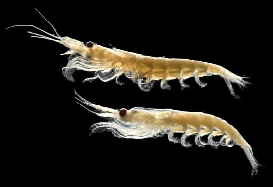
I have the privilege of studying the largest animals on the planet: blue whales (Balaenoptera musculus). However, in order to understand the ecology, distribution, and habitat use patterns of these ocean giants, I have dedicated the past several months to studying something much smaller: krill (Nyctiphanes australis). New Zealand’s South Taranaki Bight region (“STB”, Figure 1) is an important foraging ground for a unique population of blue whales [1,2]. A wind-driven upwelling system off of Kahurangi Point (the “X” in Figure 1) generates productivity in the region [3], leading to an abundance of krill [4], the desired blue whale prey [5].

Our blue whale research team collected a multitude of datastreams in three different years, including hydroacoustic data to map krill distribution throughout our study region. The summers of 2014 and 2017 were characterized by what could be considered “typical” conditions: A plume of cold, upwelled water curving its way around Cape Farewell (marked with the star in Figure 1) and entering the South Taranaki Bight, spurring a cascade of productivity in the region. The 2016 season, however, was different. The surface water temperatures were hot, and the whales were not where we expected to find them.

Figure 2. Sea surface temperature maps of the South Taranaki Bight region in each of our three study years. The white circles indicate where most blue whale sightings were made in each year. Note the very warm temperatures in 2016, and more westerly location of blue whale sightings.

What happened to the blue whales’ food source under these different conditions in 2016? Before I share some preliminary findings from my recent analyses, it is important to note that there are many possible ways to measure krill availability. For example, the number of krill aggregations, as well as how deep, thick, and dense those aggregations are in an area will all factor into how “desirable” krill patches are to a blue whale. While there may not be “more” or “less” krill from one year to the next, it may be more or less accessible to a blue whale due to energetic costs of capturing it. Here is a taste of what I’ve found so far:

In 2016, when surface waters were warm, the krill aggregations were significantly deeper than in the “typical” years (ANOVA, F=7.94, p <0.001):

Figute 3. Boxplots comparing the median krill aggregation depth in each of our three survey years.

The number of aggregations was not significantly different between years, but as you can see in the plot below (Figure 4) the krill were distributed differently in space:

Figure 4. Map of the South Taranaki Bight region with the number of aggregations per 4 km^2, standardized by vessel survey effort. The darker colors represent areas with a higher density of krill aggregations. 

While the bulk of the krill aggregations were located north of Cape Farewell under typical conditions (2014 and 2017), in the warm year (2016) the krill were not in this area. Rather, the area with the most aggregations was offshore, in the western portion of our study region. Now, take a look at the same figure, overlaid with our blue whale sighting locations:

Figure 5. Map of standardized number of krill aggregations, overlaid with blue whale sighting locations in red stars.

Where did we find the whales? In each year, most whale encounters were in the locations where the most krill aggregations were found! Not only that, but in 2016 the whales responded to the difference in krill distribution by shifting their distribution patterns so that they were virtually absent north of Cape Farewell, where most sightings were made in the typical years.

The above figures demonstrate the importance of studying an ecosystem. We could puzzle and speculate over why the blue whales were further west in the warm year, but the story that is emerging in the krill data may be a key link in our understanding of how the ecosystem responds to warm conditions. While the focus of my dissertation research is blue whales, they do not live in isolation. It is through understanding the ecosystem-scale story that we can better understand blue whale ecology in the STB. As I continue modeling the relationships between oceanography, krill, and blue whales in warm and typical years, we are beginning to scratch the surface of how blue whales may be responding to their environment.

  1. Torres LG. 2013 Evidence for an unrecognised blue whale foraging ground in New Zealand. New Zeal. J. Mar. Freshw. Res. 47, 235–248. (doi:10.1080/00288330.2013.773919)
  2. Barlow DR et al. 2018 Documentation of a New Zealand blue whale population based on multiple lines of evidence. Endanger. Species Res. 36, 27–40. (doi:https://doi.org/10.3354/esr00891)
  3. Shirtcliffe TGL, Moore MI, Cole AG, Viner AB, Baldwin R, Chapman B. 1990 Dynamics of the Cape Farewell upwelling plume, New Zealand. New Zeal. J. Mar. Freshw. Res. 24, 555–568. (doi:10.1080/00288330.1990.9516446)
  4. Bradford-Grieve JM, Murdoch RC, Chapman BE. 1993 Composition of macrozooplankton assemblages associated with the formation and decay of pulses within an upwelling plume in greater cook strait, New Zealand. New Zeal. J. Mar. Freshw. Res. 27, 1–22. (doi:10.1080/00288330.1993.9516541)
  5. Gill P. 2002 A blue whale (Balaenoptera musculus) feeding ground in a southern Australian coastal upwelling zone. J. Cetacean Res. Manag. 4, 179–184.

Understanding sea otter effects through complexity

By Dominique Kone, Masters Student in Marine Resource Management

Species reintroductions are a management strategy to augment the reestablishment or recovery of a locally-extinct or extirpated species into once native habitat. The potential for reestablishment success often depends on the species’ ecological characteristics, habitat requirements, and relationship and effects to other species in the environment[1]. While the science behind species reintroductions is continuously evolving and improving, reintroductions are still inherently risky and uncertain in nature. Therefore, every effort should be made to fully assess ecological factors before a reintroduction takes place. As Oregon considers a potential sea otter reintroduction, understanding these ecological factors is an important piece of my own graduate research.

Sea otters are oftentimes referred to as keystone species because they can have wide-reaching effects on the community structure and function of nearshore marine environments. Furthermore, relative to other marine mammals or top predators, several papers have documented these effects – partially due to the ease in observing their foraging and social behaviors, which typically take place close to shore. In many of these studies, a classic paradigm repeatedly appears: when sea otters are present, prey densities (e.g., sea urchins) are significantly reduced, while macroalgae (e.g., kelp, seagrass) densities are high.

Source: Belleza.

While this paradigm is widely-accepted amongst researchers, a few key studies have also demonstrated that the effects of sea otters may be more variable than we once thought. The paradigm does not necessarily hold true everywhere sea otters exist, or at least not to the same degree. For example, after observing benthic communities along islands with varying sea otter densities in the Aleutian archipelago, Alaska, researchers found that islands with abundant otter populations consistently supported low sea urchin densities and high, yet variable, kelp densities. In contrast, islands without otters consistently had low kelp densities and high, yet variable, urchin densities[2]. This study demonstrates that while the classic paradigm generally held true, the degree to which the ecosystem belonged to one of two dominant states (sea otters, low urchins, and high kelp or no sea otters, high urchins, and low kelp) was less obvious.

This example demonstrates the danger in applying this one-size-fits-all paradigm to sea otter effects. Hence, we want to achieve a better understanding of potential sea otter effects so that managers may anticipate how Oregon’s nearshore environments may be affected if sea otters were to be reintroduced. Yet, how can we accurately anticipate these effects given these potential variations and deviations from the paradigm? Interestingly, if we look to other fields outside ecology, we find a possible solution and tool for tackling these uncertainties: a systematic review of available literature.

Two ecosystem states as predicted by the classic paradigm (left: kelp-dominated; right: urchin-dominated). Source: SeaOtters.com.

For decades, medical researchers have been conducting systematic reviews to assess the efficacy of treatments and drugs by combining several studies to find common findings[3]. These findings can then be used to determine any potential variation between studies (i.e. instances where the results may conflict or differ from one another) and even test the influence and importance of key factors that may be driving that variation[4]. While systematic reviews are quite popular within the medical research field, they have not been applied regularly in ecology, but recognition of their application to ecological questions is growing[5]. In our case of achieving a better understanding of the drivers of ecological impacts of sea otter, a systematic literature review is an ideal tool to assess variable effects. This review will be the focus of my second thesis chapter.

In conducting my review, there will be three distinct phases: (1) review design and study collection, (2) meta-analysis, and (3) factor testing. In the first phase (review design and study collection), I will search the existing literature to collect studies that explicitly compare the availability of key ecosystem components (i.e. prey species, non-prey species, and macroalgae species) when sea otters are absent and present in the environment. By only including studies that make this comparison, I will define effects as the proportional change in each species’ or organism group’s availability (e.g. abundance, biomass, density, etc.) with and without sea otters. In determining these effects, it’s important to recognize that sea otters alter ecosystems via both direct and indirect pathways. Direct effects can be thought of as any change to prey availability via sea otter predation directly, while indirect effects can be thought of an any alteration to the broader ecosystem (i.e. non-prey species, macroalgae, habitat features) as an indirect result from sea otter predation on prey species. I will record both types of effects.

General schematic of a meta-analysis in a systematic review. A meta-analysis is the process of taking multiple datasets (i.e. Data 1, Data 2 etc.) from literature sources, calculating summary statistics or effects (i.e. Summary 1, Summary 2, etc.) for each dataset, running statistical procedures (e.g. SMA = sequential meta-analysis) to relate summary effects and investigate between study variation, and identifying important features driving variation. Source: MediCeption.

In phase two, I will use meta-analytical procedures (i.e. statistical analyses specific to systematic reviews) to calculate one standardized metric to represent sea otter effects. These effects will be calculated and averaged across all collected studies. As previously discussed, there may be key factors – such as sea otter density – that influence these effects. Therefore, in phase three (factor testing), effects will also be calculated separately for each a priori factor to test their influence on the effects. Such factors may include habitat type (i.e. hard or soft sediment), prey species (i.e. sea urchins, crabs, clams, etc.), otter density, depth, or time after otter recolonization.

In statistical terms, the goal of testing factors is to see if the variation between studies is impacted by calculating sea otter effects separately for each factor versus across all studies. In other words, if we find high variation in effects between studies, there may be important factors driving that variation. Therefore, in systematic reviews, we recalculate effects separately for each factor to try to explain that variation. If, however, after testing these factors, variation remains high, there may be other factors that we didn’t test that could be driving that remaining variation. Yet, without a priori knowledge on what those factors could be, such variation should be reported as a major source of uncertainty.

Source: Giancarlo Thomae.

Predicting or anticipating the effects of reintroduced species is no easy feat. In instances where the ecological role of a species is well known – and there is adequate data – researchers can develop and use ecosystem models to predict with some certainty what these effects may be. Yet, in other cases where the species’ role is less studied, has less data, or is more variable, researchers must look to other tools – such as systematic reviews – to gain a better understanding of these potential effects. In this case, a systematic review on sea otter effects may prove particularly useful in helping managers understand what types of ecological effects of sea otters in Oregon are most likely, what the important factors are, and, after such review, what we still don’t know about these effects.

References:

[1] Seddon, P. J., Armstrong, D. P., and R. F. Maloney. 2007. Developing the science of reintroduction biology. Conservation Biology. 21(2): 303-312.

[2] Estes, J. A., Tinker, M. T., and J. L. Bodkin. 2009. Using ecological function to develop recovery criteria for depleted species: sea otters and kelp forests in the Aleutian Archipelago. Conservation Biology. 24(3): 852-860.

[3] Sutton, A. J., and J. P. T. Higgins. 2008. Recent developments in meta-analysis. Statistics in Medicine. 27: 625-650.

[4] Arnqvist, G., and D. Wooster. 1995. Meta-analysis: synthesizing research findings in ecology and evolution. TREE. 10(6): 236-240.

[5] Vetter, D., Rucker, G., and I. Storch. 2013. Meta-analysis: a need for well-defined usage in ecology and conservation biology. Ecosphere. 4(6): 1-13.

Science (or the lack thereof) in the Midst of a Government Shutdown

By Alexa Kownacki, Ph.D. Student, OSU Department of Fisheries and Wildlife, Geospatial Ecology of Marine Megafauna Lab

In what is the longest government shutdown in the history of the United States, many people are impacted. Speaking from a scientist’s point of view, I acknowledge the scientific community is one of many groups that is being majorly obstructed. Here at the GEMM Laboratory, all of us are feeling the frustrations of the federal government grinding to a halt in different ways. Although our research spans great distances—from Dawn’s work on New Zealand blue whales that utilizes environmental data managed by our federal government, to new projects that cannot get federal permit approvals to state data collection, to many of Leigh’s projects on the Oregon coast of the USA that are funded and collaborate with federal agencies—we all recognize that our science is affected by the shutdown. My research on common bottlenose dolphins is no exception; my academic funding is through the US Department of Defense, my collaborators are NOAA employees who contribute NOAA data; I use publicly-available data for additional variables that are government-maintained; and I am part of a federally-funded public university. Ironically, my previous blog post about the intersection of science and politics seems to have become even more relevant in the past few weeks.

Many graduate students like me are feeling the crunch as federal agencies close their doors and operations. Most people have seen the headlines that allude to such funding-related issues. However, it’s important to understand what the funding in question is actually doing. Whether we see it or not, the daily operations of the United States Federal government helps science progress on a multitude of levels.

Federal research in the United States is critical. Most governmental branches support research with the most well-known agencies for doing so being the National Science Foundation (NSF), the US Department of Agriculture (USDA), the National Oceanic and Atmospheric Administration (NOAA), and the National Aeronautics and Space Administration. There are 137 executive agencies in the USA (cei.org). On a finer scale, NSF alone receives approximately 40,000 scientific proposals each year (nsf.gov).

If I play a word association game and I am given the word “science”, my response would be “data”. Data—even absence data—informs science. The largest aggregate of metadata with open resources lives in the centralized website, data.gov, which is maintained by the federal government and is no longer accessible and directs you to this message:Here are a few more examples of science that has stopped in its track from lesser-known research entities operated by the federal government:

Currently, the National Weather Service (NWS) is unable to maintain or improve its advanced weather models. Therefore, in addition to those of us who include weather or climate aspects into our research, forecasters are having less and less information on which to base their weather predictions. Prior to the shutdown, scientists were changing the data format of the Global Forecast System (GFS)—the most advanced mathematical, computer-based weather modeling prediction system in the USA. Unfortunately, the GFS currently does not recognize much of the input data it is receiving. A model is only as good as its input data (as I am sure Dawn can tell you), and currently that means the GFS is very limited. Many NWS models are upgraded January-June to prepare for storm season later in the year. Therefore, there are long-term ramifications for the lack of weather research advancement in terms of global health and safety. (https://www.washingtonpost.com/weather/2019/01/07/national-weather-service-is-open-your-forecast-is-worse-because-shutdown/?noredirect=on&utm_term=.5d4c4c3c1f59)

An example of one output from the GFS model. (Source: weather.gov)

The Food and Drug Administration (FDA)—a federal agency of the Department of Health and Human Services—that is responsible for food safety, has reduced inspections. Because domestic meat and poultry are at the highest risk of contamination, their inspections continue, but by staff who are going without pay, according to the agency’s commissioner, Dr. Scott Gottlieb. Produce, dry foods, and other lower-risk consumables are being minimally-inspected, if at all.  Active research projects investigating food-borne illness that receive federal funding are at a standstill.  Is your stomach doing flips yet? (https://www.nytimes.com/2019/01/09/health/shutdown-fda-food-inspections.html?rref=collection%2Ftimestopic%2FFood%20and%20Drug%20Administration&action=click&contentCollection=timestopics&region=stream&module=stream_unit&version=latest&contentPlacement=2&pgtype=collection)

An FDA field inspector examines imported gingko nuts–a process that is likely not happening during the shutdown. (Source: FDA.gov)

The National Parks Service (NPS) recently made headlines with the post-shutdown acts of vandalism in the iconic Joshua Tree National Park. What you might not know is that the shutdown has also stopped a 40-year study that monitors how streams are recovering from acid rain. Scientists are barred from entering the park and conducting sampling efforts in remote streams of Shenandoah National Park, Virginia. (http://www.sciencemag.org/news/2019/01/us-government-shutdown-starts-take-bite-out-science)

A map of the sampling sites that have been monitored since the 1980s for the Shenandoah Watershed Study and Virginia Trout Stream Sensitivity Study that cannot be accessed because of the shutdown. (Source: swas.evsc.virginia.edu)

NASA’s Stratospheric Observatory for Infrared Astronomy (SOFIA), better known as the “flying telescope” has halted operations, which will require over a week to bring back online upon funding restoration. SOFIA usually soars into the stratosphere as a tool to study the solar system and collect data that ground-based telescopes cannot. (http://theconversation.com/science-gets-shut-down-right-along-with-the-federal-government-109690)

NASA’s Stratospheric Observatory for Infrared Astronomy (SOFIA) flies over the snowy Sierra Nevada mountains while the telescope gathers information. (Source: NASA/ Jim Ross).

It is important to remember that science happens outside of laboratories and field sites; it happens at meetings and conferences where collaborations with other great minds brainstorm and discover the best solutions to challenging questions. The shutdown has stopped most federal travel. The annual American Meteorological Society Meeting and American Astronomical Society meeting were two of the scientific conferences in the USA that attract federal employees and took place during the shutdown. Conferences like these are crucial opportunities with lasting impacts on science. Think of all the impressive science that could have sparked at those meetings. Instead, many sessions were cancelled, and most major agencies had zero representation (https://spacenews.com/ams-2019-overview/). Topics like lidar data applications—which are used in geospatial research, such as what the GEMM Laboratory uses in some its projects, could not be discussed. The cascade effects of the shutdown prove that science is interconnected and without advancement, everyone’s research suffers.

It should be noted, that early-career scientists are thought to be the most negatively impacted by this shutdown because of financial instability and job security—as well as casting a dark cloud on their futures in science: largely unknown if they can support themselves, their families, and their research. (https://eos.org/articles/federal-government-shutdown-stings-scientists-and-science). Graduate students, young professors, and new professionals are all in feeling the pressure. Our lives are based on our research. When the funds that cover our basic research requirements and human needs do not come through as promised, we naturally become stressed.

An adult and a juvenile common bottlenose dolphin, forage along the San Diego coastline in November 2018. (Source: Alexa Kownacki)

So, yes, funding—or the lack thereof—is hurting many of us. Federally-funded individuals are selling possessions to pay for rent, research projects are at a standstill, and people are at greater health and safety risks. But, also, science, with the hope for bettering the world and answering questions and using higher thinking, is going backwards. Every day without progress puts us two days behind. At first glance, you may not think that my research on bottlenose dolphins is imperative to you or that the implications of the shutdown on this project are important. But, consider this: my study aims to quantify contaminants in common bottlenose dolphins that either live in nearshore or offshore waters. Furthermore, I study the short-term and long-term impacts of contaminants and other health markers on dolphin hormone levels. The nearshore common bottlenose dolphin stocks inhabit the highly-populated coastlines that many of us utilize for fishing and recreation. Dolphins are mammals, that respond to stress and environmental hazards, in similar ways to humans. So, those blubber hormone levels and contamination results, might be more connected to your health and livelihood than at first glance. The fact that I cannot download data from ERDDAP, reach my collaborators, or even access my data (that starts in the early 1980s), does impact you. Nearly everyone’s research is connected to each other’s at some level, and that, in turn has lasting impacts on all people—scientists or not. As the shutdown persists, I continue to question how to work through these research hurdles. If anything, it has been a learning experience that I hope will end soon for many reasons—one being: for science.

Hundreds and hundreds and hundreds of models: An ecologist’s love for programming

By Dawn Barlow, PhD student, Department of Fisheries & Wildlife, Geospatial Ecology of Marine Megafauna Lab

When people hear that I study blue whales, they often ask me questions about what it’s like to be close to the largest animal on the planet, where we do fieldwork, and what data we are interested in collecting. While I love time at sea, my view on a daily basis is rarely like this:

Our small research vessel at sunset in New Zealand’s South Taranaki Bight at the end of a day of blue whale survey. Photo by D. Barlow.

More often than not, it looks something like this:

In my application letter to Dr. Leigh Torres, I wrote something along the lines of “while I relish remote fieldwork, I also find great satisfaction in the analysis process.” This statement is increasingly true for me as I grow more proficient in statistical modeling and computer programming. When excitedly telling my family about how I am trying to model relationships between oceanography, krill, whales, and satellite imagery, I was asked what I meant by “model”. Put simply, a model is a formula or equation that we can use to describe a pattern. I have been told, “all models are wrong, but some models work.” What does this mean? While we may never know exactly every pattern of whale feeding behavior, we can use the data we have to describe some of the important relationships. If our model performance is very good, then we have likely described most of what drives the patterns we see. If model performance is poor, then there is more to the pattern that we have not yet captured in either our data collection or in our analytical methods. Another common saying about models is, “A model is only ever as good as the data you put into it.” While we worked hard during field seasons to collect a myriad of data about what could be influencing blue whale distribution patterns, we inevitably could not capture everything, nor do we know everything that should be measured.

So, how do you go about finding the ‘best’ model? This question is what I’ve been grappling with over the last several weeks. My goal is to describe the patterns in the krill that drive patterns in whale distribution, the patterns in oceanography that drive patterns in the krill, and the patterns in the oceanography that drive patterns in whale distribution. The thing is, we have many metrics to describe oceanographic patterns (surface temperature, mixed layer depth, strength of the thermocline, integral of fluorescence, to name just a few), as well as several metrics to describe the krill (number of aggregations, aggregation density, depth, and thickness). When I multiplied out how many possible combinations of predictor variables and parameters we’re interested in modeling, I realized this meant running nearly 300 models in order to settle on the best ten. This is where programming comes in, I told myself, and caught my breath.

I’ve always loved languages. When I was much younger, I thought I might want to study linguistics. As a graduate student in wildlife science, the language I’ve spent the most time learning, and come to love, is the statistical programming language R. Just like any other language, R has syntax and structure. Like any other language, there are many ways in which to articulate something, to make a particular point or reach a particular end goal. Well-written code is sometimes described as “elegant”, much like a well-articulated piece of writing. While I certainly do not consider myself “fluent” in R, it is a language I love learning. I like to think that the R scripts I write are an attempt to eloquently uncover and describe ecological patterns.

Rather than running 300 models one by one, I wrote an R script to run many models at a time, and then sort the outputs by model performance. I may look at the five best models of 32 options in order to select one. But this is where Leigh reminds me to step back from the programming for a minute and put my ecologist hat back on. Insight on the part of the modeler is needed in order to discern between what are real ecological relationships and what are spurious correlations in the data. It may not be quite as simple as choosing the model with the highest explanatory power when my goal is to make ecological inferences.

So, where does this leave me? Hundreds of models later, I am still not entirely sure which ones are best, although I’ve narrowed it down considerably. My programming proficiency and confidence continue to grow, but that only goes so far in ecology. Knowledge of my study system is equally important. So my workflow lately goes something like this: write code, try to interpret model outputs, consider what I know about the oceanography of my study region, re-write code, re-interpret the revised results, and so on. Hopefully this iterative process is bringing us gradually closer to an understanding of the ecology of blue whales on a foraging ground… stay tuned.

A blue whale lunges on an aggregation of krill in New Zealand’s South Taranaki Bight. Drone piloted by Todd Chandler.

Why Feeling Stupid is Great: How stupidity fuels scientific progress and discovery

By Alexa Kownacki, Ph.D. Student, OSU Department of Fisheries and Wildlife, Geospatial Ecology of Marine Megafauna Lab

It all started with a paper. On Halloween, I sat at my desk, searching for papers that could answer my questions about bottlenose dolphin metabolism and realized I had forgotten to check my email earlier. In my inbox, there was a new message with an attachment from Dr. Leigh Torres to the GEMM Lab members, saying this was a “must-read” article. The suggested paper was Martin A. Schwartz’s 2008 essay, “The importance of stupidity in scientific research”, published in the Journal of Cell Science, highlighted universal themes across science. In a single, powerful page, Schwartz captured my feelings—and those of many scientists: the feeling of being stupid.

For the next few minutes, I stood at the printer and absorbed the article, while commenting out loud, “YES!”, “So true!”, and “This person can see into my soul”. Meanwhile, colleagues entered my office to see me, dressed in my Halloween costume—as “Amazon’s Alexa”, talking aloud to myself. Coincidently, I was feeling pretty stupid at that moment after just returning from a weekly meeting, where everyone asked me questions that I clearly did not have the answers to (all because of my costume). This paper seemed too relevant; the timing was uncanny. In the past few weeks, I have been writing my PhD research proposal —a requirement for our department— and my goodness, have I felt stupid. The proposal outlines my dissertation objectives, puts my work into context, and provides background research on common bottlenose dolphin health. There is so much to know that I don’t know!

Alexa dressed as “Amazon Alexa” on Halloween at her office in San Diego, CA.

When I read Schwartz’s 2008 paper, there were a few takeaway messages that stood out:

  1. People take different paths. One path is not necessarily right nor wrong. Simply, different. I compared that to how I split my time between OSU and San Diego, CA. Spending half of the year away from my lab and my department is incredibly challenging; I constantly feel behind and I miss the support that physically being with other students provides. However, I recognize the opportunities I have in San Diego where I work directly with collaborators who teach and challenge me in new ways that bring new skills and perspective.

    Image result for different ways
    (Image source: St. Albert’s Place)
  2. Feeling stupid is not bad. It can be a good feeling—or at least we should treat it as being a positive thing. It shows we have more to learn. It means that we have not reached our maximum potential for learning (who ever does?). While writing my proposal I realized just how little I know about ecotoxicology, chemistry, and statistics. I re-read papers that are critical to understanding my own research, like “Nontargeted biomonitoring of halogenated organic compounds in two ecotypes of bottlenose dolphins (Tursiops truncatus) from the Southern California bight” (2014) by Shaul et al. and “Bottlenose dolphins as indicators of persistent organic pollutants in the western north Atlantic ocean and northern gulf of Mexico” (2011) by Kucklick et al. These articles took me down what I thought were wormholes that ended up being important rivers of information. Because I recognized my knowledge gap, I can now articulate the purpose and methods of analysis for specific compounds that I will conduct using blubber samples of common bottlenose dolphins

    Image result
    Image source: memegenerator.net
  3. Drawing upon experts—albeit intimidating—is beneficial for scientific consulting as well as for our mental health; no one person knows everything. That statement can bring us together because when people work together, everyone benefits. I am also reminded that we are our own harshest critics; sometimes our colleagues are the best champions of our own successes. It is also why historical articles are foundational. In the hunt for the newest technology and the latest and greatest in research, it is important to acknowledge the basis for discoveries. My data begins in 1981, when the first of many researchers began surveying the California coastline for common bottlenose dolphins. Geographic information systems (GIS) were different back then. The data requires conversions and investigative work. I had to learn how the data were collected and how to interpret that information. Therefore, it should be no surprise that I cite literature from the 1970s, such as “Results of attempts to tag Atlantic Bottlenose dolphins, (Tursiops truncatus)” by Irvine and Wells. Although published in 1972, the questions the authors tried to answer are very similar to what I am looking at now: how are site fidelity and home ranges impacted by natural and anthropogenic processes. While Irvine and Wells used large bolt tags to identify individuals, my project utilizes much less invasive techniques (photo-identification and blubber biopsies) to track animals, their health, and their exposures to contaminants.

    Image result for that is why you fail yoda
    (Image source: imgflip.com)
  4. Struggling is part of the solution. Science is about discovery and without the feeling of stupidity, discovery would not be possible. Feeling stupid is the first step in the discovery process: the spark that fuels wanting to explore the unknown. Feeling stupid can lead to the feeling of accomplishment when we find answers to those very questions that made us feel stupid. Part of being a student and a scientist is identifying those weaknesses and not letting them stop me. Pausing, reflecting, course correcting, and researching are all productive in the end, but stopping is not. Coursework is the easy part of a PhD. The hard part is constantly diving deeper into the great unknown that is research. The great unknown is simultaneously alluring and frightening. Still, it must be faced head on. Schwartz describes “productive stupidity [as] being ignorant by choice.” I picture this as essentially blindly walking into the future with confidence. Although a bit of an oxymoron, it resonates the importance of perseverance and conviction in the midst of uncertainty.

    Image result for funny t rex
    (Image source: Redbubble)

Now I think back to my childhood when stupid was one of the forbidden “s-words” and I question whether society had it all wrong. Maybe we should teach children to acknowledge ignorance and pursue the unknown. Stupid is a feeling, not a character flaw. Stupidity is important in science and in life. Fascination and emotional desires to discover new things are healthy. Next time you feel stupid, try running with it, because more often than not, you will learn something.

Image may contain: 1 person, sitting, table, child and outdoor
Alexa teaching about marine mammals to students ages 2-6 and learning from educators about new ways to engage young students. San Diego, CA in 2016. (Photo source: Lori Lowder)

[B]reaching New Discoveries about Gray Whales in Oregon

By Haley Kent, Marine Studies Initiative (MSI) & summer GEMM Lab intern, OSU senior

“BLOW!”, yells a team “Whale Storm” member, as mist remains above the water from an exhaling gray whale (Eschrichtius robustus). While based at the Port Orford Field Station for 6 weeks of my final summer as an undergrad at Oregon State University my heart has only grown fonder for marine wildlife. I am still in awe of this amazing opportunity of researching the foraging ecology of gray whales as a Marine Studies Initiative and GEMM Lab intern. From this field work I have already learned so much about gray whales and their zooplankton prey, and now it’s time to analyze the data we have collected and see what ecological stories we can uncover.

Figure 1. Robyn and Haley enjoy their time in the research kayak. Photo by Lisa Hildebrand.

WORK IN THE FIELD

This internship is my first field work experience and I have learned many skills and demands needed to study marine wildlife: waking up before the sun (every day begins with screaming alarms), being engulfed by nature (Port Orford is a jaw-dropping location with rich biodiversity), packing up damp gear and equipment to only get my feet wet in the morning ocean waves again, and of course waiting on the weather to cooperate (fog, wind, swell). I wouldn’t want it any other way.

Figure 2. Smokey sunrise from the research kayak. Photo by Haley Kent.

Whether it is standing above the ocean on the ‘Cliff Site’ or sitting in our two-man kayak, every day of this internship has been full of new learning experiences. Using various field work techniques, such as using a theodolite (surveying equipment to track whale location and behavior), Secchi disks (to measure water clarity), GoPro data collection, taking photos of wildlife, and many more tools, have given me a new bank of valuable skills that will stick with me into my future career.

Figure 3. Haley drops Secchi disk from the research kayak. Photo by Dylan Gregory.

Data Analysis

To maximize my amazing internship experience, I am conducting a small data analysis project using the data we have collected these past weeks and in previous summers.  There are so many questions that can be asked of these data, but I am particularly interested in how many times individual gray whales return to our study area to forage seasonally or annually, and if these individual whales forage preferentially where certain zooplankton prey are available.

Photo Identification

After many hours of data collection in the field either in the kayak or on the cliff, we get to take a breather in the lab to work on various projects we are each assigned. Some job tasks include processing data, identifying zooplankton, and looking through the photos taken that day to potentially identify a known whale. Once photos are processed and saved onto the rugged laptop, they are ready for some serious one on one. Looking through each of the 300 photos captured each day can be very tedious, but it is worthwhile when a match is found. Within the photos of each individual whale I first determine whether it is the left or right side of the whale – if we are lucky we get both! – and maybe even a fluke (tail) photo!

Figure 4. Buttons’ left side. Photo taken by Gray Whale Team of 2018.
Figure 5. Buttons’ left side. Photo taken by Gray Whale Team of 2017.

The angles of these photos (Fig. 4 & 5) are very different, so it could be difficult to tell these are the same whale. But, have a closer look at the pigmentation patterns on this whale. Focus on a single spot or area of spots, and see how patterns line up. Does that match in the same area in the next photo? If yes, you could have yourself a match!

Buttons, one of the identified gray whales (Fig. 4 & 5), was seen in 2016, 17, and 18. I was so excited to identify Buttons for the 3rd year in a row as this result demonstrates this whale’s preference for foraging in Port Orford.

Zooplankton and whale foraging behavior

By using the theodolite we track the whale’s position from the cliff location. I have plugged these coordinates into Google Earth, and compared the coordinates to our zooplankton sample stations from that same day. These methods allow me to assess where the whale spent time, and where it did not, which I can then relate to the zooplankton species and abundance we caught in our sample tows (we use a net from the research kayak to collect samples throughout the water column).

Figure 6. Holmesimysis sculpta. This species can range between 4-12mm. The size of this zooplankton relative to the large gray whales foraging on it shows the whale’s incredible senses for prey preference. Photo source: Scripps Institute of Oceanography.

Results (preliminary)

‘Eyeball’ is one of our resident whales that we have identified regularly throughout this season here in Port Orford. I have compared the amount of time Eyeball has spent near zooplankton stations to the prey community we captured at each station.

There is a positive trend in the amount of time the whale spent in an area with the percent abundance of Holmesimysis sculpta (Fig. 7: blue trend line).

Figure 7. Comparative plot between the amount of time the whale “Eyeball” spent within 50m of each zooplankton sampling station and the relative amount of zooplankton species caught at each station. Note the positive trend between time and Holmesimysis sculpta, and the negative trend relative to Neomysis sp. or Caprellidae.

Conversely, there is an inverse trend with two other zooplankton species:  Neomysis sp. (grey trend line) and Caprellidae (orange trend line). These results suggest that Eyeball has a foraging preference for areas where Holmesimysis sculpta (Fig. 6) is more abundant. Who would have known a whale could be so picky? Once the season comes to an end, I plan to use more of our data to continue to make discoveries about the foraging preferences of gray whales in Oregon.

Cloudy with a chance of blue whales

By Dawn Barlow, PhD student, Department of Fisheries & Wildlife, Geospatial Ecology of Marine Megafauna Lab

As a PhD student studying the ecology of blue whales in New Zealand, my time is occupied by questions such as: When and where are the blue whales? Can we predict where they will be based on environmental conditions? How does their distribution overlap with human activity such as oil and gas exploration?

Leigh and I have just returned from New Zealand, where I gave an oral presentation at the Society for Conservation Biology Oceania Congress entitled “Cloudy with a chance of whales: Forecasting blue whale presence to mitigate industrial impacts based on tiered, bottom-up models”. While the findings I presented are preliminary, an exciting ecological story is emerging, and one with clear management implications.

The South Taranaki Bight (STB) region of New Zealand is an important area for a population of blue whales which are unique to New Zealand. A wind-driven upwelling system brings cold, productive waters into the bight [1], which sustains high densities of krill [2], blue whale prey. The region is also frequented by busy shipping traffic, oil and gas drilling and extraction platforms as well as seismic survey effort for subsurface oil and gas reserves, and is the site of a recently-permitted seabed mine for iron sands (Fig. 1). However, a lack of knowledge on blue whale distribution and habitat use patterns has impeded effective management of these potential anthropogenic threats.

Figure 1. A blue whale surfaces in front of a floating production storage and offloading vessel servicing the oil rigs in the South Taranaki Bight. Photo by D. Barlow.

Three surveys were conducted in the STB region in the summer months of 2014, 2016, and 2017. During that time, we not only looked for blue whales, we also collected oceanographic data and hydroacoustic backscatter data to map and measure aspects of the krill in the region. These data streams will help us understand the functional, ecological relationships between the environment (oceanography), prey (krill), and predators (blue whales) in the ecosystem (Fig. 2). But in practice these data are costly and time-consuming to collect, while other data sources such as satellite imagery are readily accessible to managers at a variety of spatial and temporal scales. Therefore, another one of my aims is to link the data we collected in the field to satellite imagery, so that managers can have a practical tool to predict when and where the blue whales are most likely to be found in the region.

Figure 2. Data streams collected during surveys of the South Taranaki Bight Region in 2014, 2016, and 2017. 

So what did I find? Here are the highlights from my preliminary analyses:

  • The majority of the patterns in blue whale distribution can be explained by the density, depth, and thickness of the krill patches.
  • Patterns in the krill are driven by oceanography.
  • Those same oceanographic parameters that drive the krill can be used to explain blue whale distribution.
  • There are tight relationships between the important oceanographic variables and satellite images of sea surface temperature.
  • Blue whale distribution can, to some degree, be explained using just satellite imagery.

We were able to identify a sea surface temperature range in the satellite imagery of approximately 18°C where the likelihood of finding a blue whale is the highest. Is this because blue whales really like 18° water? Well, more likely this relationship exists because the satellite imagery is reflective of the oceanography, and the oceanography drives patterns in the krill distribution, and the krill drives the distribution of blue whales (Fig. 3). We were able to make each of these functional linkages through our series of models, which is quite exciting.

Figure 3. The tiered modeling approach we took to investigate the ecological relationships between blue whales, krill, oceanography, and satellite imagery. Because of the ecological linkages we made, we are able to say that any relationship between whale distribution and satellite imagery most likely reflects a relationship between the blue whales and their prey. 

That’s all well and good, but we were interested in testing these relationships to see if our identified habitat associations hold up even when we do not have field data (oceanographic, krill, and whale data). This past austral summer, we did not have a field season to collect data, but there was a large seismic airgun survey of the STB region. Seismic survey vessels are required to have trained marine mammal observers on board, and we were given access to the blue whale sightings data they recorded during the survey. In December, when the water was right around the preferred temperature identified by our models (18°C), the observers made 52 blue whale sightings (Fig. 4). In January and February, the waters warmed and only two sightings were made in each month. This is not only reassuring because it supports our model results, it also implies that there is the potential to balance industrial use of the area with protection of blue whale habitat, based on our understanding of the ecology. In January and February, very few blue whales were likely disturbed by the industrial activity in the STB, as conditions were not favorable for foraging at the location of the seismic survey. In contrast, the blue whales that were in the STB region in December may have experienced physiological consequences of sustained exposure to airgun noise since the conditions were favorable for foraging in the STB. In other words, the whales may have tolerated the noise exposure to gain access to good food, but this could have significant biological repercussions such as increased stress [3].

Figure 4. Monthly sea surface temperature (MODIS Aqua) overlaid with blue whale sightings from marine mammal observers aboard seismic survey vessel R/V Amazon Warrior. Black rectangles represent areas of seismic survey effort. Blue whale sighting location data were provided by RPS Energy Pty Ltd & Schlumberger, and Todd Energy.

In the first two weeks of July, we presented these latest findings to managers at the New Zealand Department of Conservation, the Minister of Conservation, the CEO and Policy Advisor of a major oil and gas conglomerate, NGOs, advocacy groups, and scientific colleagues. It was valuable to gather feedback from many different stakeholders, and satisfying to see such a clear interest in, and management application of, our work.

Dr. Leigh Torres and Dawn Barlow in front of Parliament in Wellington, New Zealand, following the presentation of their recent findings.

What’s next? We’re back in Oregon, and diving back into analysis. We intend to take the modeling work a step further to make the models predictive—for example, can we forecast where the blue whales will be based on the temperature, productivity, and winds two weeks prior? I am excited to see where these next steps lead!

References:

  1. Shirtcliffe TGL, Moore MI, Cole AG, Viner AB, Baldwin R, Chapman B. 1990 Dynamics of the Cape Farewell upwelling plume, New Zealand. New Zeal. J. Mar. Freshw. Res. 24, 555–568. (doi:10.1080/00288330.1990.9516446)
  2. Bradford-Grieve JM, Murdoch RC, Chapman BE. 1993 Composition of macrozooplankton assemblages associated with the formation and decay of pulses within an upwelling plume in greater cook strait, New Zealand. New Zeal. J. Mar. Freshw. Res. 27, 1–22. (doi:10.1080/00288330.1993.9516541)
  3. Rolland RM, Parks SE, Hunt KE, Castellote M, Corkeron PJ, Nowacek DP, Wasser SK, Kraus SD. 2012 Evidence that ship noise increases stress in right whales. Proc. Biol. Sci. 279, 2363–8. (doi:10.1098/rspb.2011.2429)

Forecasting blue whale presence: Small steps toward big goals

By Dawn Barlow, MSc student, Department of Fisheries and Wildlife, Geospatial Ecology of Marine Megafauna Lab

In 2013, Leigh first published a hypothesis that the South Taranaki Bight region between New Zealand’s North and South Islands is important habitat for blue whales  (Torres 2013). Since then, we have collected three years of data and conducted dedicated analyses, so we now understand that a unique population of blue whales is found in New Zealand, and that they are present in the South Taranaki Bight year-round (Barlow et al. in press).

A blue whale surfaces in the South Taranaki Bight. Photo by Leigh Torres.

This research has garnered quite a bit of political and media attention. A major platform item for the New Zealand Green Party around the last election was the establishment of a marine mammal sanctuary in the South Taranaki Bight. When the world’s largest seismic survey vessel began surveying the South Taranaki Bight this summer for more oil and gas reserves using tremendously loud airguns, there were rallies on the lawn in front of Parliament featuring a large inflatable blue whale that the protesters affectionately refer to as “Janet”. Needless to say, blue whales have made their way into the spotlight in New Zealand.

Janet the inflatable blue whale accompanies protesters on the lawn in front of Parliament in Wellington, New Zealand. Image credit: Greenpeace.

Now that we know there is a unique population of blue whales in New Zealand, what is next? What’s next for me is an exciting combination of both ecology and conservation. If an effective sanctuary is to be implemented, it needs to be more than a simple box drawn on a map to check off a political agenda item—the sanctuary should be informed by our best ecological knowledge of the blue whales and their habitat.

In July, Leigh and I will attend the Society for Conservation Biology meeting in Wellington, New Zealand, and I’ll be giving a presentation titled “Cloudy with a chance of whales: Forecasting blue whale presence based on tiered, bottom-up models”. I’ll be the first to admit, I am not yet forecasting blue whale presence. But I am working my way there, step-by-step, through this tiered, bottom-up approach. In cetacean habitat modeling, we often assume that whale distribution on a foraging ground is determined by their prey’s distribution, and that satellite images of temperature and chlorophyll-a provide an accurate picture of what is going on below the surface. Is this true? With our three years of data including in situ oceanography, krill hydroacoustics, and blue whale distribution and behavior, we are in a unique position to test some of those assumptions, as well as provide managers with an informed management tool to predict blue whale distribution.

What questions will we ask using our data? Firstly, can in situ oceanography (i.e., thermocline depth and temperature, mixed layer depth) predict the distribution and density of blue whale prey (krill)? Then, can those prey patterns be accurately predicted in the absence of oceanographic measurements, using just satellite images? Next, we’ll bring the blue whales back into the picture to ask: can we predict blue whale distribution based on our in situ measurements of oceanography and prey? And finally, in the absence of in situ measurements (which is most often the case), can we forecast where the whales will be based just on remotely-sensed images of the region?

The transducer pole in the water off the RV Star Keys (left) deployed with the echosounder to collect prey availability data, including this image (right) of krill swarms near feeding blue whales. Photo by Leigh Torres.

So, cloudy with a chance of whales? Well, you’ll have to stay tuned for that story in the coming months. In the meantime, I can tell you that as daunting as it is to aggregate so many data streams, each step of the way has a piece of the story to tell. I can’t wait to see how it falls together, both from an ecological modeling perspective and a conservation management objective.

A blue whale surfaces in front of a floating production storage and offloading (FPSO) vessel which services the oil rigs in the South Taranaki Bight. Photo by Dawn Barlow.


References:

Torres, L. G. (2013). Evidence for an unrecognised blue whale foraging ground in New Zealand. New Zealand Journal of Marine and Freshwater Research47(2), 235-248.

Barlow, D. R., Torres, L. G., Hodge, K. B., Steel, D. Baker, C. S., Chandler, T. E., Bott, N., Constantine, R., Double, M. C., Gill, P., Glasgow, D., Hamner, R. M., Lilley, C., Ogle, M., Olson, P. A., Peters, C., Stockin, K. A., Tessaglia-Hymes, C. T., Klinck, H. (in press). Documentation of a New Zealand blue whale population based on multiple lines of evidence. Endangered Species Research. 

The Land of Maps and Charts: Geospatial Ecology

By Alexa Kownacki, Ph.D. Student, OSU Department of Fisheries and Wildlife, Geospatial Ecology of Marine Megafauna Lab

I love maps. I love charts. As a random bit of trivia, there is a difference between a map and a chart. A map is a visual representation of land that may include details like topology, whereas a chart refers to nautical information such as water depth, shoreline, tides, and obstructions.

Map of San Diego, CA, USA. (Source: San Diego Metropolitan Transit System)
Chart of San Diego, CA, USA. (Source: NOAA)

I have an intense affinity for visually displaying information. As a child, my dad traveled constantly, from Barrow, Alaska to Istanbul, Turkey. Immediately upon his return, I would grab our standing globe from the dining room and our stack of atlases from the coffee table. I would sit at the kitchen table, enthralled at the stories of his travels. Yet, a story was only great when I could picture it for myself. (I should remind you, this was the early 1990s, GoogleMaps wasn’t a thing.) Our kitchen table transformed into a scene from Master and Commander—except, instead of nautical charts and compasses, we had an atlas the size of an overgrown toddler and salt and pepper shakers to pinpoint locations. I now had the world at my fingertips. My dad would show me the paths he took from our home to his various destinations and tell me about the topography, the demographics, the population, the terrain type—all attribute features that could be included in common-day geographic information systems (GIS).

Uncle Brian showing Alexa where they were on a map of Maui, Hawaii, USA. (Photo: Susan K. circa 1995)

As I got older, the kitchen table slowly began to resemble what I imagine the set from Master and Commander actually looked like; nautical charts, tide tables, and wind predictions were piled high and the salt and pepper shakers were replaced with pencil marks indicating potential routes for us to travel via sailboat. The two of us were in our element. Surrounded by visual and graphical representations of geographic and spatial information: maps. To put my map-attraction this in even more context, this is a scientist who grew up playing “Take-Off”, a board game that was “designed to teach geography” and involved flying your fleet of planes across a Mercator projection-style mapboard. Now, it’s no wonder that I’m a graduate student in a lab that focuses on the geospatial aspects of ecology.

A precocious 3-year-old Alexa, sitting with the airplane pilot asking him a long list of travel-related questions (and taking his captain’s hat). Photo: Susan K.

So why and how did geospatial ecology became a field—and a predominant one at that? It wasn’t that one day a lightbulb went off and a statistician decided to draw out the results. It was a progression, built upon for thousands of years. There are maps dating back to 2300 B.C. on Babylonian clay tablets (The British Museum), and yet, some of the maps we make today require highly sophisticated technology. Geospatial analysis is dynamic. It’s evolving. Today I’m using ArcGIS software to interpolate mass amounts of publicly-available sea surface temperature satellite data from 1981-2015, which I will overlay with a layer of bottlenose dolphin sightings during the same time period for comparison. Tomorrow, there might be a new version of software that allows me to animate these data. Heck, it might already exist and I’m not aware of it. This growth is the beauty of this field. Geospatial ecology is made for us cartophiles (map-lovers) who study the interdependency of biological systems where location and distance between things matters.

Alexa’s grandmother showing Alexa (a very young cartographer) how to color in the lines. Source: Susan K. circa 1994

In a broader context, geospatial ecology communicates our science to all of you. If I posted a bunch of statistical outputs in text or even table form, your eyes might glaze over…and so might mine. But, if I displayed that same underlying data and results on a beautiful map with color-coded symbology, a legend, a compass rose, and a scale bar, you might have this great “ah-ha!” moment. That is my goal. That is what geospatial ecology is to me. It’s a way to SHOW my science, rather than TELL it.

Would you like to see this over and over again…?

A VERY small glimpse into the enormous amount of data that went into this map. This screenshot gave me one point of temperature data for a single location for a single day…Source: Alexa K.

Or see this once…?

Map made in ArcGIS of Coastal common bottlenose dolphin sightings between 1981-1989 with a layer of average sea surface temperatures interpolated across those same years. A picture really is worth a thousand words…or at least a thousand data points…Source: Alexa K.

For many, maps are visually easy to interpret, allowing quick message communication. Yet, there are many different learning styles. From my personal story, I think it’s relatively obvious that I’m, at least partially, a visual learner. When I was in primary school, I would read the directions thoroughly, but only truly absorb the material once the teacher showed me an example. Set up an experiment? Sure, I’ll read the lab report, but I’m going to refer to the diagrams of the set-up constantly. To this day, I always ask for an example. Teach me a new game? Let’s play the first round and then I’ll pick it up. It’s how I learned to sail. My dad described every part of the sailboat in detail and all I heard was words. Then, my dad showed me how to sail, and it came naturally. It’s only as an adult that I know what “that blue line thingy” is called. Geospatial ecology is how I SEE my research. It makes sense to me. And, hopefully, it makes sense to some of you!

Alexa’s dad teaching her how to sail. (Source: Susan K. circa 2000)
Alexa’s first solo sailboat race in Coronado, San Diego, CA. Notice: Alexa’s dad pushing the bow off the dock and the look on Alexa’s face. (Source: Susan K. circa 2000)
Alexa mapping data using ArcGIS in the Oregon State University Library. (Source: Alexa K circa a few minutes prior to posting).

I strongly believe a meaningful career allows you to highlight your passions and personal strengths. For me, that means photography, all things nautical, the great outdoors, wildlife conservation, and maps/charts.  If I converted that into an equation, I think this is a likely result:

Photography + Nautical + Outdoors + Wildlife Conservation + Maps/Charts = Geospatial Ecology of Marine Megafauna

Or, better yet:

? + ⚓ + ? + ? + ? =  GEMM Lab

This lab was my solution all along. As part of my research on common bottlenose dolphins, I work on a small inflatable boat off the coast of California (nautical ✅, outdoors ✅), photograph their dorsal fin (photography ✅), and communicate my data using informative maps that will hopefully bring positive change to the marine environment (maps/charts ✅, wildlife conservation✅). Geospatial ecology allows me to participate in research that I deeply enjoy and hopefully, will make the world a little bit of a better place. Oh, and make maps.

Alexa in the field, putting all those years of sailing and chart-reading to use! (Source: Leila L.)


What REALLY is a Wildlife Biologist?

By Alexa Kownacki, Ph.D. Student, OSU Department of Fisheries and Wildlife, Geospatial Ecology of Marine Megafauna Lab

The first lecture slide. Source: Lecture1_Population Dynamics_Lou Botsford

This was the very first lecture slide in my population dynamics course at UC Davis. Population dynamics was infamous in our department for being an ultimate rite of passage due to its notoriously challenging curriculum. So, when Professor Lou Botsford pointed to his slide, all 120 of us Wildlife, Fish, and Conservation Biology majors, didn’t know how to react. Finally, he announced, “This [pointing to the slide] is all of you”. The class laughed. Lou smirked. Lou knew.

Lou knew that there is more truth to this meme than words could express. I can’t tell you how many times friends and acquaintances have asked me if I was going to be a park ranger. Incredibly, not all—or even most—wildlife biologists are park rangers. I’m sure that at one point, my parents had hoped I’d be holding a tiger cub as part of a conservation project—that has never happened. Society may think that all wildlife biologists want to walk in the footsteps of the famous Steven Irwin and say thinks like “Crikey!”—but I can’t remember the last time I uttered that exclamation with the exception of doing a Steve Irwin impression. Hollywood may think we hug trees—and, don’t get me wrong, I love a good tie-dyed shirt—but most of us believe in the principles of conservation and wise-use A.K.A. we know that some trees must be cut down to support our needs. Helicoptering into a remote location to dart and take samples from wild bear populations…HA. Good one. I tell myself this is what I do sometimes, and then the chopper crashes and I wake up from my dream. But, actually, a scientist staring at a computer with stacks of papers spread across every surface, is me and almost every wildlife biologist that I know.

The “dry lab” on the R/V Nathaniel B. Palmer en route to Antarctica. This room full of technology is where the majority of the science takes place. Drake Passage, International Waters in August 2015. Source: Alexa Kownacki

There is an illusion that wildlife biologists are constantly in the field doing all the cool, science-y, outdoors-y things while being followed by a National Geographic photojournalist. Well, let me break it to you, we’re not. Yes, we do have some incredible opportunities. For example, I happen to know that one lab member (eh-hem, Todd), has gotten up close and personal with wild polar bear cubs in the Arctic, and that all of us have taken part in some work that is worthy of a cover image on NatGeo. We love that stuff. For many of us, it’s those few, memorable moments when we are out in the field, wearing pants that we haven’t washed in days, and we finally see our study species AND gather the necessary data, that the stars align. Those are the shining lights in a dark sea of papers, grant-writing, teaching, data management, data analysis, and coding. I’m not saying that we don’t find our desk work enjoyable; we jump for joy when our R script finally runs and we do a little dance when our paper is accepted and we definitely shed a tear of relief when funding comes through (or maybe that’s just me).

A picturesque moment of being a wildlife biologist: Alexa and her coworker, Jim, surveying migrating gray whales. Piedras Blancas Light Station, San Simeon, CA in May 2017. Source: Alexa Kownacki.

What I’m trying to get at is that we accepted our fates as the “scientists in front of computers surrounded by papers” long ago and we embrace it. It’s been almost five years since I was a senior in undergrad and saw this meme for the first time. Five years ago, I wanted to be that scientist surrounded by papers, because I knew that’s where the difference is made. Most people have heard the quote by Mahatma Gandhi, “Be the change that you wish to see in the world.” In my mind, it is that scientist combing through relevant, peer-reviewed scientific papers while writing a compelling and well-researched article, that has the potential to make positive changes. For me, that scientist at the desk is being the change that he/she wish to see in the world.

Scientists aboard the R/V Nathaniel B. Palmer using the time in between net tows to draft papers and analyze data…note the facial expressions. Antarctic Peninsula in August 2015. Source: Alexa Kownacki.

One of my favorite people to colloquially reference in the wildlife biology field is Milton Love, a research biologist at the University of California Santa Barbara, because he tells it how it is. In his oh-so-true-it-hurts website, he has a page titled, “So You Want To Be A Marine Biologist?” that highlights what he refers to as, “Three really, really bad reasons to want to be a marine biologist” and “Two really, really good reasons to want to be a marine biologist”. I HIGHLY suggest you read them verbatim on his site, whether you think you want to be a marine biologist or not because they’re downright hilarious. However, I will paraphrase if you just can’t be bothered to open up a new tab and go down a laugh-filled wormhole.

Really, Really Bad Reasons to Want to be a Marine Biologist:

  1. To talk to dolphins. Hint: They don’t want to talk to you…and you probably like your face.
  2. You like Jacques Cousteau. Hint: I like cheese…doesn’t mean I want to be cheese.
  3. Hint: Lack thereof.

Really, Really Good Reasons to Want to be a Marine Biologist:

  1. Work attire/attitude. Hint: Dress for the job you want finally translates to board shorts and tank tops.
  2. You like it. *BINGO*
Alexa with colleagues showing the “cool” part of the job is working the zooplankton net tows. This DOES have required attire: steel-toed boots, hard hat, and float coat. R/V Nathaniel B. Palmer, Antarctic Peninsula in August 2015. Source: Alexa Kownacki.

In summary, as wildlife or marine biologists we’ve taken a vow of poverty, and in doing so, we’ve committed ourselves to fulfilling lives with incredible experiences and being the change we wish to see in the world. To those of you who want to pursue a career in wildlife or marine biology—even after reading this—then do it. And to those who don’t, hopefully you have a better understanding of why wearing jeans is our version of “business formal”.

A fieldwork version of a lab meeting with Leigh Torres, Tom Calvanese (Field Station Manager), Florence Sullivan, and Leila Lemos. Port Orford, OR in August 2017. Source: Alexa Kownacki.