By Mattea Holt Colberg, GEMM Lab summer intern, OSU junior
Science is about asking new questions in order to make new discoveries. Starting every investigation with a question, sparked by an observation, is enshrined in the scientific method and pursued by researchers everywhere. Asking questions goes beyond scientific research though; it is the best way to learn new things in any setting.
When I first arrived in Port Orford, I did not know much about gray whales. The extent of my knowledge was that they are large baleen whales that migrate every year and feed on plankton. I did, however, know quite a bit about killer whales. I have been interested in killer whales since I was 5 years old, so I have spent years reading about, watching, and listening to them (my current favorite book about them is Of Orcas and Men, by David Neiwert and I highly recommend it!). I have also had opportunities to research them in the Salish Sea, both on a sailing trip and through the dual-enrollment program Ocean Research College Academy, where I explored how killer whales respond to ambient underwater noise for a small independent project. Knowing more about killer whales than other species has caused killer whales to be the lens through which I approach learning and asking questions about other whales.
Figure 1a. Killer whales traveling in a group in the Salish Sea. Source: ISTOCK.
Figure 1b. A gray whale traveling solo in Tichenor Cove. Source: GEMM Lab.
At first, I was not sure how to apply what I know about killer whales specifically to research on gray whales, since killer whales are toothed whales, while gray whales are baleen whales. There are several differences between toothed whales and baleen whales; toothed whales tend to be more social, occurring in pods or groups, eat larger prey like fish, squid, and seals, and they echolocate. In comparison, baleen whales are less social, eat mostly tiny zooplankton prey, and do not echolocate. Because of these differences, I wanted to learn more about gray whales, so I started asking Lisa questions. Killer whales only sleep with half of their brain at a time, so I asked if gray whales do the same. They do. Killer whales typically travel in stable, long-term matriarchal groups, and I recently learned that gray whales frequently travel alone (though not exclusively). This new knowledge to me led me to ask if gray whales vocalize while traveling. They typically do not. Through asking these questions, and others, I have begun to learn more about gray whales.
Figure 2. Mattea on the tandem research kayak taking a break in between prey sampling. Source: L. Hildebrand.
I am still learning about marine mammal research, and from what I have experienced so far, marine mammal acoustics intrigues me the most. As a child, I developed a general interest in whale vocalizations after hearing recordings of them in museums and aquariums. Then, two years ago, I heard orcas vocalizing in the wild, and I decided I wanted to learn more about their vocalizations as a long-term career goal.
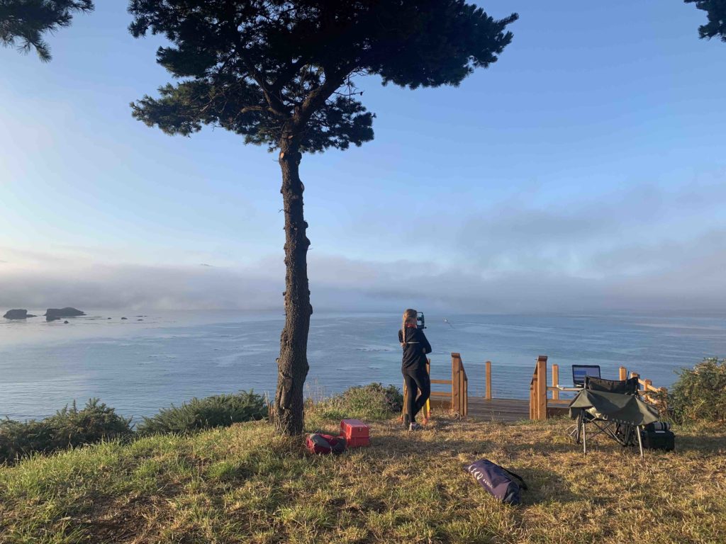
To pursue a career studying marine mammal acoustics, I will need scientific and communication skills that this internship is helping me develop. Sitting on the cliff for hours at a time, sometimes with gray whales swimming in our view-scape and sometimes without, is teaching me the patience and attention needed to review hours of sound recordings with or without vocalizations. Identifying and counting zooplankton most days is teaching me the importance of processing data regularly, so it does not build up or get too confusing, as well as attention to detail and keeping focused. Collecting data from a kayak is teaching me how to assess ocean conditions, keep track of gear, and stay calm when things go wrong. I am also practicing the skill of taking and identifying whale photos, which can be applied to many whale research topics I hope to pursue. Through writing this blog post and discussing the project with Lisa and my fellow interns, I am improving my science communication skills.
Figure 3. Mattea manning the theodolite watching and waiting for a gray whale to show up in our study area. Source: L. Hildebrand.
As an undergraduate student, it can sometimes be difficult to find opportunities to research marine mammals, so I am very grateful for and excited about this internship, both because of the skills it is helping me build and the field work experiences that I enjoy participating in. Another aspect of research this internship is helping me learn about is to ask engaging questions. As I mentioned at the beginning of this post, asking questions is a key element of conducting research. By asking questions about gray whales based on both prior knowledge and new observations, I am practicing this skill, as well as thinking of topics I am curious about and might want to explore in the future. While watching for whales, I have thought of questions such as: How is whale behavior affected by surface conditions? Do gray whales prefer feeding at certain times of the day? Questions like these help me learn about whales, and they keep me excited about research. Thanks to this internship, I can continue working towards my dreams of pursuing similar questions about whales as a career.
Yodel-Ay-Ee-Ooooo! Hello from the Theyodelers, this year’s Port Orford gray whale foraging ecology field team. In case you were wondering, no, we aren’t hobby yodelers and we don’t plan on becoming them. The team name this year actually has to be attributed to a parent of one of my interns. Shout out to Scott Holt who during the first week of the field season asked his daughter Mattea (our OSU undergraduate intern) whether using a theodolite (the instrument we use to track gray whales from our cliff site) is anything like yodeling. The name was an immediate hit with the team and so the team name discussion was closed fairly early on in the season. Now that I have explained our slightly unconventional team name, let me tell you a little about this year’s team and what has been going on down here on the Oregon south coast so far.
As you can tell from the byline, I (Lisa) am back as the project’s team lead in this, the 6th year of the Port Orford gray whale research and internship project. Going into this year’s field season with two years of experience under my belt has made me feel more confident and comfortable with diving straight back into our fine-scale research with a new team of interns. Yet, I am beginning to realize that no matter how much experience I have, there will always be unforeseeable curve balls thrown at me that I can’t anticipate no matter how prepared or experienced I am. However, my knowledge and experience now certainly inform how I tackle these curve balls and hopefully allow my problem-solving to be better and quicker. I am so thrilled that Leigh and I were able to get the field season approved here in Port Orford despite the ongoing pandemic. There were many steps we had to take and protocols to write and get approved, but it was worth the work. It certainly is strange living in a place that is meant to be your home for six weeks but having to wear a face covering everywhere except your own bedroom. However, mask wearing, frequent hand washing, and disinfecting is a very small price to pay to avoid having a lapse in our gray whale data collected here in Port Orford (and minimize transmission). Doing field research amidst COVID has certainly been a big curve ball this year but, so far, I have been able to handle these added challenges pretty well, especially with a lot of help from my team. Speaking of which, time to introduce the other Theyodelers…
Figure 1. Noah watching and waiting for whales on the cliff. When we are outside in the wind and are able to maintain a minimum 6-ft distance, we are able to remove our face coverings. Source: T. McCambridge.
First up, we have Noah Dolinajec. Noah is a fellow graduate student who is currently doing a Master’s in Marine & Lacustrine Science and Management at the Vrije Universiteit Brussel in Brussels, Belgium. While he is attending graduate school in Belgium, Noah is not actually from this European country. In fact, he is a Portlandian! As an Oregonian with a passion for the marine environment, Noah is no stranger to the Oregon coast and has spent quite some time exploring it in the past. Some other things about Noah: before going to college he played semi-professional ice hockey, he is a bit of a birder, and he likes to cook (he and I have been tag-teaming the team cooking this year).
Figure 2. Mattea outside the field station holding local fisher-pup Jim.Source: L. Hildebrand.
Next, we have Mattea Holt Colberg. As I mentioned before, Mattea is the team’s OSU undergraduate intern this year. By participating in a running-start program at her high school where she took two years of college classes, Mattea entered OSU as a junior at just 18 years old! However, she has decided to somewhat extend her undergraduate career at OSU by completing a dual major in Biology and Music. She plays the piano and the violin (which she brought to Port Orford, but we have yet to be serenaded by her). Mattea has previously conducted field research on killer whales in the Salish Sea and I can tell that she is hoping for killer whales to show up in Port Orford (while not entirely ludicrous, the chance of this happening is probably very, very slim).
Figure 3. Liz in the bow of the kayak in Tichenor Cove.Source: L. Hildebrand.
Last but certainly not least, is Liz Kelly, our Pacific High School intern from Port Orford. Liz has lived in several different states across the country (I’m talking Kentucky to Florida) and so I am really excited that she currently lives here in Oregon because she has been an absolute joy to have on the team so far. Liz brings a lot of energy and humor to the team, which we have certainly needed whenever those curve balls come flying. Besides her positivity, Liz brings a lot of determination and perseverance and seeing her work through tough situations here already has made me very proud. I really hope this internship provides Liz with the life, STEM, and communication skills she needs to help her succeed in pursuing her goals of doing wildlife research after college. As you may have read in my last blog, our previous high school interns have had successes in being admitted to various colleges to follow their goals, and I feel confident that Liz will be no different. When she is not here at the field station, she can probably be found taking care of and riding one of her four horses (Millie, Maricja, Miera, and Jeanie).
Now that I have introduced the 2020 field team, here is a short play-by-play of what we have been seeing, or perhaps more aptly, not seeing. Our whale sighting numbers have been pretty low so far and when we do see them, they seem to be foraging a little further away from our study site than I am used to seeing in past years. However, this shift in behavior is not entirely surprising to me since our zooplankton net has been coming up pretty empty at our sampling stations. While there are mysids and amphipods scattered here and there, their numbers are in the low 10s when we do our zooplankton ID lab work in the afternoons. These low counts are also reflected by the low densities I am anecdotally seeing on our GoPro drops (Fig 4).
Figure 4. Comparison of zooplankton density from our GoPro videos. Both images were taken at the same sampling station (Tichenor Cove 8), however the image on the left that contains a lot of little critters is from 2018, whereas the image on the right is from last week. This year our drops have been looking more like the image on the right, though typically with even fewer zooplankton.
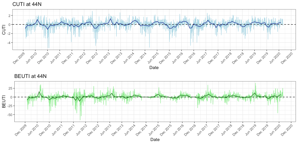
While I am not entirely certain why we are seeing this low prey abundance, I do have some hypotheses. The most likely reason is that this year we experienced some delayed upwelling on our coast. Dawn wrote a great blog about upwelling and wind a few weeks ago and I suggest checking it out to better understand what upwelling is and how it can affect whales (and the whole ecosystem). Typically, we see our peak upwelling occur here in Oregon in May-June. However, if you look at Figure 5 you will see that both the indices remained low at that time this year, whereas in previous years, they were already increasing by May/June.
Figure 5. 10 year time series of the Coastal Upwelling Transport Index (CUTI; top plot) and Biologically Effective Upwelling Transport Index (BEUTI; bottom plot) at 44ºN. CUTI represents the amount of upwelling (positive numbers) or downwelling (negative numbers) while BEUTI estimates the amount of nitrate (i.e. nutrients) upwelled (positive numbers) and downwelled (negative numbers). The light-colored lines representthe CUTI and BEUTI at that point in time while the dark, bold lines represent the long-term average.
A delayed upwelling means that there was likely less nutrients in the water to support little critters like zooplankton to start reproducing and increasing their abundances. Simply put, it means our coastal waters appear to be less productive than they usually are at this time of the year. If there is not much prey around (as we have been finding in our two study sites – Mill Rocks and Tichenor Cove), then it makes sense to me why gray whales are not hanging around since there is not much to feed on. Fortunately, the tail of the trend line in Figure 5 is angling upward, which means that the upwelling finally started in June so hopefully the nutrients, zooplankton and whales will follow soon too. In fact, since I wrote the draft of this blog at the end of last week, we have actually seen an increase in the numbers of mysids in our zooplankton net and on our GoPro videos.
We are almost halfway done with the field season already and I cannot believe how quickly it goes by! During the first two weeks we were busy getting familiar with all of our gear and completing First Aid/CPR and kayak paddle & rescue courses. This week the team started the real data collection. We have had some hiccups (we lost our GoPro stick and our backup GoPro stick, but thankfully have already recovered one of them) but overall, we are off to a pretty good start. Now we just need the upwelling to really kick in, for there to be thick layers of mysids, and for the whales to come in close. Over the next three weeks, you will be hearing from Noah, Mattea and Liz as they share their experiences and viewpoints with all of you!
Clara Bird, Masters Student, OSU Department of Fisheries and Wildlife, Geospatial Ecology of Marine Megafauna Lab
The field season can be quite a hectic time of year. Between long days out on the water, trouble-shooting technology issues, organizing/processing the data as it comes in, and keeping up with our other projects/responsibilities, it can be quite overwhelming and exhausting.
But despite all of that, it’s an incredible and exciting time of year. Outside of the field season, we spend most of our time staring at our computers analyzing the data that we spend a relatively short amount of time collecting. When going through that process it can be easy to lose sight of why we do what we do, and to feel disconnected from the species we are studying. Oftentimes the analysis problems we encounter involve more hours of digging through coding discussion boards than learning about the animals themselves. So, as busy as it is, I find that the field season can be pretty inspiring. I have recently been looking through our most recent drone footage of gray whales and feeling renewed excitement for my thesis.
At the moment, my thesis has four central questions: (1) Are there associations between habitat type and gray whale foraging tactic? (2) Is there evidence of individualization? (3) What is the relationship between behavior and body condition? (4) Do we see evidence of learning in the behavior of mom and calf pairs? As I’ve been organizing my thoughts, what’s become quite clear is how interconnected these questions are. So, I thought I’d take this blog to describe the potential relationships.
Let’s start with the first question: are there associations between habitat types and gray whale foraging tactics? This question is central because it relates foraging behavior to habitat, which is ultimately associated with prey. This relationship is the foundation of all other questions involving foraging tactics because food is necessary for the whales to have the energy and nutrients they need to survive. It’s reasonable to think that the whales are flexible and use different foraging tactics to eat different prey that live in different habitats. But, if different prey types have different nutritional value (this is something that Lisa is studying right now; check out the COZI project to learn more), then not all whales may be getting the same nutrients.
The next question relates to the first question but is not necessarily dependent on it. It’s the question of individualization, a topic Lisa also explored in a past blog. Within our Oregon field sites we have documented a variety of gray whale foraging tactics (Torres et al. 2018; Video 1) but we do not know if all gray whales use all the tactics or if different individuals only use certain tactics. While I think it’s unlikely that one whale only uses one tactic all the time, I think we could see an individual use one tactic more often than the others. I reason that there could be two reasons for this pattern. First, it could be a response to resource availability; certain tactics are more efficient than others, this could be because the tactic involves capturing the more nutritious prey or because the behavior is less energetically demanding. Second, foraging tactics are socially learned as calves from their mothers, and hence individuals use those learned tactics more frequently. This pattern of maternally inherited foraging tactics has been documented in other marine mammals (Mann and Sargeant 2009; Estes et al. 2003). These questions between foraging tactic, habitat and individualization also tie into the remaining two questions.
My third question is about the relationship between behavior and body condition. As I’ve discussed in a previous blog, I am interested in assessing the relative energetic costs and benefits of the different foraging tactics. Is one foraging tactic more cost-effective than another (less energy out per energy in)? Ever since our lab’s cetacean behavioral ecology class, I’ve been thinking about how my work relates to niche partitioning theory (Pianka 1974).This theory states that when there is low prey availability, niche partitioning will increase. Niche partitioning can occur across several different dimensions: for instance, prey type, foraging location, and time of day when active. If gray whales partition across the prey type dimension, then different whales would feed on different kinds of prey. If whales partition resources across the foraging location dimension, individuals would feed in different areas. Lastly, if whales partition resources across the time axis, individuals would feed at different times of day. Using different foraging tactics to feed on different prey would be an example of partitioning across the prey type dimension. If there is a more preferable prey type, then maybe in years of high prey availability, we would see most of the gray whales using the same tactics to feed on the same prey type. However, in years of low prey availability we might expect to see a greater variety of foraging tactics being used. The question then becomes, does any whale end up using the less beneficial foraging tactic? If so, which whales use the less beneficial tactic? Do the same individuals always switch to the less beneficial tactic? Is there a common characteristic among the individuals that switched, like sex, age, size, or reproductive status? Lemos et al. (2020) hypothesized that the decline in body condition observed from 2016 to 2017 might be a carryover effect from low prey availability in 2016. Could it be that the whales that use the less beneficial tactic exhibit poor body condition the following year?
My fourth, and final, question asks if foraging tactics are passed down from moms to their calves. We have some footage of a mom foraging with her calf nearby, and occasionally it looks like the calf could be copying its mother. Reviewing this footage spiked my interest in seeing if there are similarities between the behavior tactics used by moms and those used by their calves after they have been weaned. While this question clearly relates to the question of individualization, it is also related to body condition: what if the foraging tactics used by the mom is influenced by her body condition at the time?
I hope to answer some of these fascinating questions using the data we have collected during our long field days over the past 6 years. In all likelihood, the story that comes together during my thesis research will be different from what I envision now and will likely lead to more questions. That being said, I’m excited to see how the story unfolds and I look forward to sharing the evolving ideas and plot lines with all of you.
References
Estes, J A, M L Riedman, M M Staedler, M T Tinker, and B E Lyon. 2003. “Individual Variation in Prey Selection by Sea Otters: Patterns, Causes and Implications.” Source: Journal of Animal Ecology. Vol. 72.
Mann, Janet, and Brooke Sargeant. 2009. “ Like Mother, like Calf: The Ontogeny of Foraging Traditions in Wild Indian Ocean Bottlenose Dolphins ( Tursiops Sp.) .” In The Biology of Traditions, 236–66. Cambridge University Press. https://doi.org/10.1017/cbo9780511584022.010.
Pianka, Eric R. 1974. “Niche Overlap and Diffuse Competition” 71 (5): 2141–45.
Soledade Lemos, Leila, Jonathan D Burnett, Todd E Chandler, James L Sumich, and Leigh G. Torres. 2020. “Intra‐ and Inter‐annual Variation in Gray Whale Body Condition on a Foraging Ground.” Ecosphere 11 (4). https://doi.org/10.1002/ecs2.3094.
Torres, Leigh G., Sharon L. Nieukirk, Leila Lemos, and Todd E. Chandler. 2018. “Drone up! Quantifying Whale Behavior from a New Perspective Improves Observational Capacity.” Frontiers in Marine Science 5 (SEP). https://doi.org/10.3389/fmars.2018.00319.
By Alejandro Fernandez Ajo, PhD student at the Department of Biology, Northern Arizona University, Visiting scientist in the GEMM Lab working on the gray whale physiology and ecology project
Two years ago, in August 2018, I came to Newport and visited the Hatfield Marine Science Center for the first time with an NSF/RCN-founded laboratory exchange with the GEMM Lab and met Dr. Leigh Torres. My goals during this exchange where to learn about non-invasive fieldwork techniques for studying free-range whales while interacting, exchanging ideas, and networking with the GEMM Lab members; also, to discuss some projects and thoughts for future collaborations with Dr. Torres. During those two weeks in Newport, I had the opportunity to help with field work on the project “Evaluation of gray whale ecology and physiology in response to variable ambient ocean noise conditions”, which aims to evaluate the hormonal variability and health of the gray whales that forage along the Oregon coast in the context of multiple stressors. I would return during the summers of 2019 and 2020 as a visiting scientist and research assistant to work on this project. This year the experience has been a bit different in terms of interactions with the HMSC community due to COVID-19; however, we were able to successfully start the field season in time and now we are wrapping up our second month of surveys with many new and interesting data gathered, and many new, unforgettable memories to be treasured. Working with these animals is incredibly fascinating because there are so many things we don´t know about them, and the questions can become both overwhelming and exciting.
An essential part of this project, and arguably any research project done with cetaceans, is the identification of individuals. Hence, considerable effort is expended each year attempting to photograph every gray whale possible within our study region and to identify each whale we encounter. The GEMM Lab maintains a catalog of the gray whales that visit the Oregon coast, a sub-population known as the Pacific Coast Feeding Group (PCFG). This catalog currently consists of 173 individuals. which we frequently compare with a larger catalog of gray whales that includes 2060 individuals observed since 1977 (Cascadia Research Collective). These methods allow us to know who is who among the whales we encounter each day at sea.
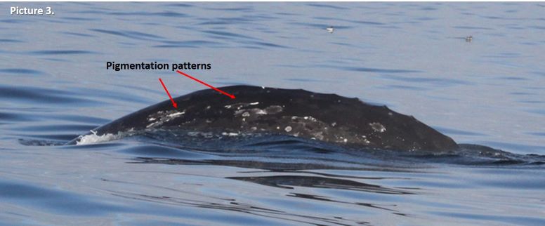
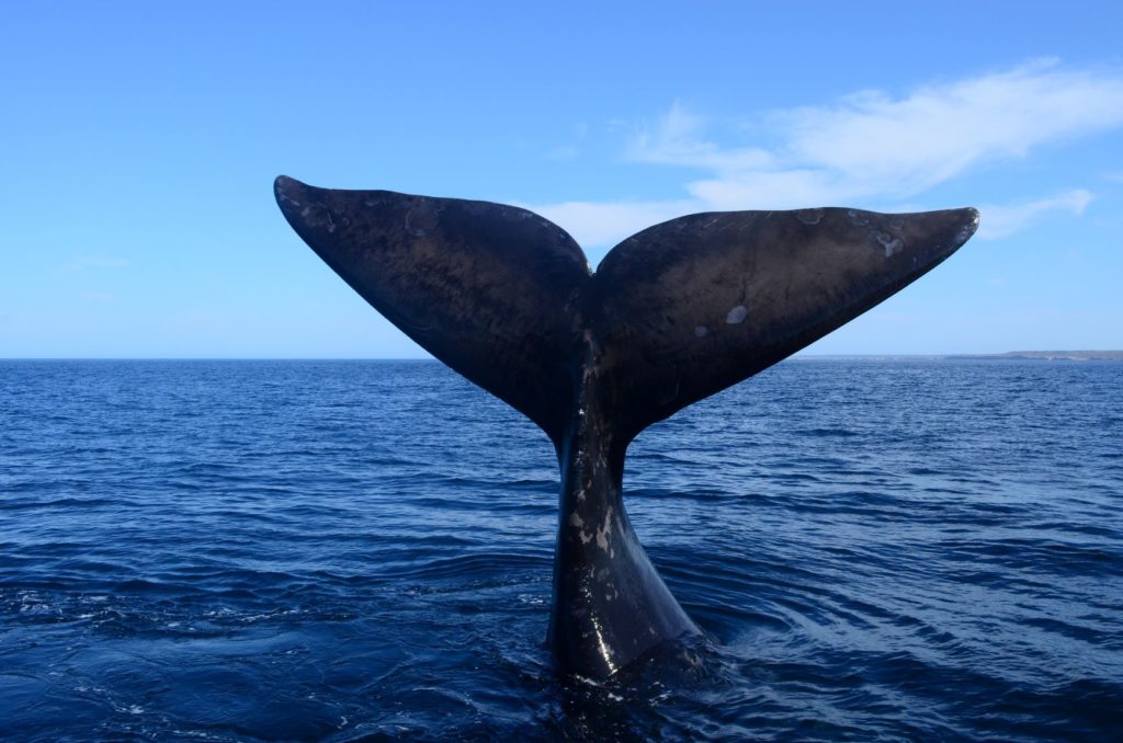
The different species of cetaceans can be individually identified by markings on their bodies, very much like fingerprints in humans. Some features on these animals are unique and conserved through life. For example, Southern and Northern right whales are identified by the callosity patters in their heads (Picture 1), while humpback whales are mostly identified individually by the shape and the patterns of black and white pigmentation on the underside of their fluke (Picture 2). Gray whales have very mottled skin coloration, so we use a combination of markings and features to identify individuals: pigmentation patterns, scars, shape and pigmentation of their fluke, and sometimes the shape of their knuckles, which are a series of “humps” that gray whales have instead of a dorsal fin on their back. It might sound very difficult to do, and it can be a tedious task, however as you train your eye it becomes easier, and features that at first seemed undistinguishable become recognizable and unique (Picture 3). As a reward, it is such a joy to find a match and recognize old friends when they arrive from their long journeys in the vast ocean each year to the Oregon coast.
The callosity pattern of a southern right whale.Photo by Alejandro Fernández Ajó – Instituto de Conservación de Ballenas.Three different humpback whales with notably different pigmentation patterns on their flukes. Photographs captured under NOAA/NMFS permit #21678.The gray whale “Knife” we have observed frequently this summer off the Oregon coast. Can you see how the right pigmentation pattern identified looks like a knife? Photograph captured under NOAA/NMFS permit #21678.
As a result of our photo-identification efforts and the high site-fidelity of the whales we study, the large majority of the gray whales we observe here in Oregon are known individually. For many whales, we also have detailed sightings records that can span years and decades, that document calving history, lactation, appearance of scars indicative of injury or entanglement, minimum age, sex, habitat-use patterns, behaviors, etc. Holding such detailed information of individual whales provides incredible contributions to our understanding of the basic patterns in life history of whales, such as reproduction rates, calving intervals, age of first reproduction, etc. Moreover, when these life history events are linked with physiological sample collection large steps can be made in the development and validation of physiological methods. Many endocrine assays currently in use for whales are based on non-traditional sample types including feces, respiratory vapor, and baleen, which have been validated using the catalogs of well-known individuals to verify that measured hormones reflect patterns expected for various physiological states. For example, we can compare endocrine data of confirmed pregnant females, known mature males, and known-injured whales to learn how whale physiological responses are different during different life history events (e.g., Burgess et al. 2017, 2018, Corkeron et al. 2017, Hunt et al. 2006, 2016, 2018, Lysiak et al. 2018, Rolland et al. 2005).
Here in Oregon we are learning from the lives of the gray whales we study, and here I want to share with you two of their stories, one happy and one not-so-happy.
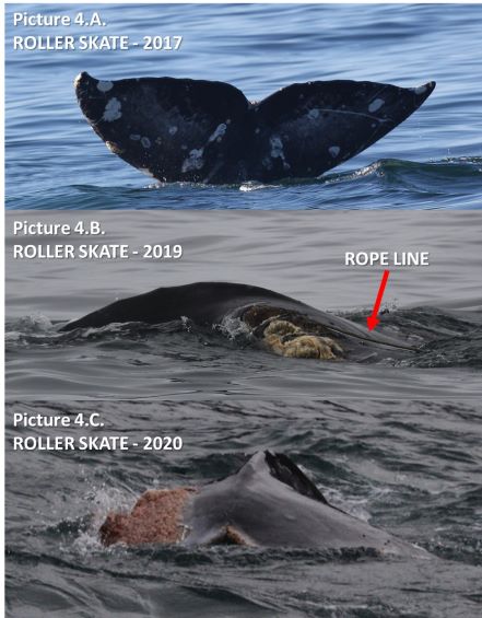
Let´s start with the not-so-happy story so we can end with some brighter news. On June 24 this year, we encountered a whale near Cape Foulweather, which is a very tricky area to work as there are many rocks and shallow water that make the sea conditions very choppy even with low swell. We started documenting the sighting as usual, taking pictures of the left side, the right side and ideally also the fluke of the whale. As we approached this whale, we started noting that something was wrong with its fluke. With the challenging sea conditions, it was not easy to approach the whale and the whale was not exposing its fluke when diving. When we put our drone up to collect photogrammetry and behavior data we gained a much better perspective. This whale has a bad injury on it fluke (Picture 4.C). On the boat we started making conjectures about the cause of this terrible injury that had basically amputate most of its left fluke lobe. Once back on shore, we sorted out the photos and compared the field images captured during the day with the photo-ID catalog and we made a match. This whale is known in our catalog as “ROLLER SKATE”, is a female, and was first sighted in 2015, so she is at least 5 years old today.
The story unfolded when we reviewed Roller Skate’s sighting history. Interestingly we observed this same whale in the same location last September 2019. Unfortunately, it was a very brief encounter but enough for photo documentation of the whale and an interesting observation. Here I quote the field notes that Dr. Torres wrote from this sighting: “September 6th, 2019. Sighting 9: Scattered whales feeding and/or traveling across area to north of Cape Foulweather. One whale had recently chopped fluke; tried to re-find to get better photos but could not (looking at photos now, this whale is clearly entangled in line!). Ceiling too low for UAS [drone flight].” (Picture 4.B).
Progressive photos of Roller Skate’s fluke. In 2017, her fluke was healthy (A). In 2019, we observed her fluke with a line entanglement and “chewed up” (B). In 2020, we have observed the resulting wound and healing process (C). Photographs captured under NOAA/NMFS permit #21678.
Roller skate’s story is an example of how essential is to keep an ID catalog. After a close-up examination of the 2019 picture, we can clearly see a rope entanglement (Picture 4.B). Photos from previous years show how beautiful and healthy her fluke was before this event (Picture 4.A). This event is heart breaking to witness, but this whale could be considered lucky because she was able to shed the gear and survive this entanglement, at least in the short term. Additionally, we can learn from Roller Skate’s misfortune to help us understand what the consequences of such an injury (stressor) may be on the physiology of a whale. We have been eager to collect a fecal sample from Roller Skate to analyze how her hormone levels compare to non-injured whales. Fortunately, we got lucky a couple weeks ago and collected this sample, so now we need to get in the lab and analyze the samples. But more questions remain: Will this injury impact her ability to reproduce? If so, for how long? And at a larger scale, what are the population consequences of such events? If we can understand the magnitude of lethal and sublethal human caused impacts on individual whales and their populations from events such as entanglements, we can develop better methods to mitigate and limit such hazards for whales in their environments.
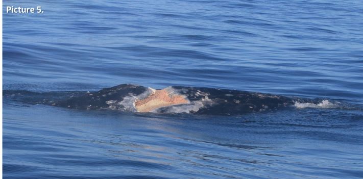
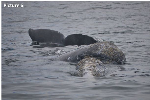
As I promised, there is also some good news to share. A very well-known PCFG whale, almost a celebrity I dear to say, is “Scarback”, or as we like to call her “Scarlett”. Scarlett is a female known since 1996, making her at least 24 years old, and she also has a very bad injury of unknown origin. Scarlett has a terrible scar on her back that is theorized to have been caused by an explosive harpoon, or maybe a bad ship-strike (Picture 5), but we really do not know. However, we do know she survived this injury and this year she brought a new calf into the population (Picture 6). This is the second calf we have documented from Scarlett, with her previous calf sighted during the 2016 field season and we call it “Brown”. Scarlett is an example of how resilient these amazing giants can be; however, it is likely that while she was recovering from this injury, she was unable to reproduce. How many calves from Scarlett did the PCFG population “lose” due to such a tragedy? We can´t know, but we are learning, and her story will also help us understand whale physiology as we will analyze her fecal hormones and body condition during pregnancy, lactation, and resting phases.
The scar on Scarlett’s back. This significant wound has an unknown origin.Photograph captured under NOAA/NMFS permit #21678.
Scarlett is a survivor. We need to recognize that we are sharing the ocean with different forms of life. We need to acknowledge their existence and understand how our use of the oceans is affecting them, and, more importantly, work toward improving their conditions. I hope that with our research we highlight and communicate how amazing are these animals, and how important are they for marine ecosystems. And ultimately, I hope our work helps minimize the impacts that affect other forms of ocean life that coexist with us, both above and below the surface.
The well-known gray whale “Scarlett” surfaces under her calf while it checks out the GEMM Lab field team. Photo by Alejandro Fernandez Ajo taken under NOAA/NMFS permit #21678.
References:
Burgess, E., Hunt, K. E., Kraus, S. D. and Rolland, R. M. (2016). Get the most out of blow hormones: validation of sampling materials, field storage and extraction techniques for whale respiratory vapor samples. Conservation Physiology, 4, cow024.
Burgess, E. A., Hunt, K. E., Kraus, S. D. and Rolland, R. M. (2018). Quantifying hormones in exhaled breath for physiological assessment of large whales at sea. Scientific Reports, 8, 10031.
Corkeron, P. J., Rolland, R. M., Hunt, K. E. and Kraus, S. D. (2017). A right whale PooTree: Fecal hormones and classification trees identify reproductive states in North Atlantic right whales (Eubalaena glacialis). Conservation Physiology, 5, cox006. DOI: 10.1093/conphys/cox006.
Hunt, K., Lysiak, N., Moore, M. and Rolland, R. (2017). Multi-year longitudinal profiles of cortisol and corticosterone recovered from baleen of North Atlantic right whales (Eubalaena glacialis). General and Comparative Endocrinology, 254, 50-59. DOI: 10.1016/j.ygcen.2017.09.009.
Hunt, K., Lysiak, N. S. J., Matthews, C. J. D., et al. (2018). Multi-year patterns in testosterone, cortisol and corticosterone in baleen from adult males of three whale species. Conservation Physiology, 6, coy049. DOI: 10.1093/conphys/coy049.
Hunt, K. E., Rolland, R. M., Kraus, S. D. and Wasser, S. K. (2006). Analysis of fecal glucocorticoids in the North Atlantic Right Whale (Eubalaena glacialis). General and Comparative Endocrinology, 148, 260-272.
Lysiak, N., Trumble, S., Knowlton, A. and Moore, M. (2018). Characterizing the duration and severity of fishing gear entanglement on a North Atlantic right whale (Eubalaena glacialis) using stable isotopes, steroid and thyroid hormones in baleen. Frontiers in Marine Science. DOI: 10.3389/fmars.2018.00168.
Rolland, R. M., Hunt, K. E., Kraus, S. D. and Wasser, S. K. (2005). Assessing reproductive status of right whales (Eubalaena glacialis) using fecal hormone metabolites. General and Comparative Endocrinology, 142, 308-317.
By: Alexa Kownacki, Ph.D. Student, OSU Department of Fisheries and Wildlife, Geospatial Ecology of Marine Megafauna Lab
Humans are fascinated by food. We want to know its source, its nutrient content, when it was harvested and by whom, and so much more. Since childhood, I was the nagging child who interrogated wait staff about the seafood menu because I cared about the sustainability aspect as well as consuming ethically-sourced seafood. Decades later I still do the same: ask a myriad of questions from restaurants and stores in order to eat as sustainably as possible. But in addition to asking these questions about my food, I also question what my study species eats and why. My study populations, common bottlenose dolphins, are described as top opportunistic predators (Norris and Prescott 1961, Shane et al. 1986, Barros and Odell 1990). In my study area off of California, this species exists in two ecotypes. The coastal ecotype off of California, USA are generalist predators, feeding on many different species of fish using different foraging techniques (Ballance 1992, Shane 1990). The offshore ecotype, on the other hand, is less well-studied, but is frequently observed in association with sperm whales, although the reason is still unknown (Díaz-Gamboa et al. 2018). Stable isotope analysis from skin samples from the two ecotypes indicates that the ecotypes exhibit different foraging strategies based on different isotopic carbon and nitrogen levels (Díaz-Gamboa et al. 2018).
Growing up, I kept the Monterey Bay Aquarium’s Seafood Watch Guide with me to choose the most sustainably-sourced seafood at restaurants. Today there is an easy-to-use application for mobile phones that replaced the paper guide. (Image Source: https://www.seafoodwatch.org/)
Preliminary and historical data on common bottlenose dolphins (Tursiops truncatus) suggest that the coastal ecotype spend more time near estuary mouths than offshore dolphins (Ballance 1992, Kownacki et al. unpublished data). Estuaries contain large concentrations of nutrients from runoff, which support zooplankton and fishes. It is for this reason that these estuaries are thought to be hotspots for bottlenose dolphin foraging. Some scientists hypothesize that these dolphins are estuarine-based prey specialists (Barros and Odell 1990), or that the dolphins simply aggregate in estuaries due to higher prey abundance (Ballance 1992).
Coastal bottlenose dolphins traveling near an estuary mouth in San Diego, CA. (Photographed under NOAA NMFS Permit # 19091).
In an effort to understand diet compositions of bottlenose dolphins, during coastal surveys seabirds were recorded in association with feeding groups of dolphins. Therefore, it is reasonable to believe that dolphins were feeding on the same fishes as Brown pelicans, blue-footed and brown boobies, double-crested cormorants, and magnificent frigatebirds, seeing as they were the most common species associated with bottlenose dolphin feeding groups (Ballance 1992). A shore-based study by Hanson and Defran (1993) found that coastal dolphins fed more often in the early morning and late afternoon, as well as during periods of high tide current. These patterns may have to do with the temporal and spatial distribution of prey fish species. From the few diet studies conducted on these bottlenose dolphins in this area, 75% of the prey were species from the families Ebiotocidae (surf perches) and Sciaendae (croakers) (Norris and Prescott 1961, Walker 1981). These studies, in addition to optimal foraging models, suggest this coastal ecotype may not be as much of a generalist as originally suggested (Defran et al. 1999).
A redtail surfperch caught by a fisherman from a beach in San Diego, CA. These fish are thought to be common prey of coastal bottlenose dolphins. (Image Source: FishwithJD)
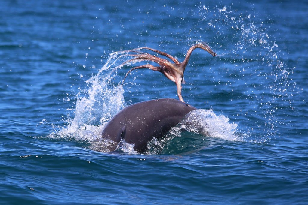
Diet studies on the offshore ecotype of bottlenose dolphins worldwide show a preference for cephalopods, similar to other toothed cetaceans who occupy similar regions, such as Risso’s dolphin, sperm whales, and pilot whales (Clarke 1986, Cockcroft and Ross 1990, Gonzalez et al. 1994, Barros et al. 2000, Walker et al. 1999). Because these animals seldom strand on accessible beaches, stomach contents analyses are limited to few studies and isotope analysis is more widely available from biopsies. We know these dolphins are sighted in deeper waters than the habitat of coastal dolphins where there are fewer nutrient plumes, so it is reasonable to hypothesize that the offshore ecotype consumes different species and may be more specialized than the coastal ecotype.
An bottlenose dolphin forages on an octopus. (Image source: Mandurah Cruises)
For a species that is so often observed from shore and boats, and is known for its charisma, it may be surprising that the diets of both the coastal and offshore bottlenose dolphins are still largely unknown. Such is the challenge of studying animals that live and feed underwater. I wish I could simply ask a dolphin, much like I would ask staff at restaurants: what is on the menu today? But, unfortunately, that is not possible. Instead, we must make educated hypotheses about the diets of both ecotypes based on necropsies and stable isotope studies, and behavioral and spatial surveys. And, I will continue to look to new technologies and creative thinking to provide the answers we are seeking.
Literature cited:
Ballance, L. T. (1992). Habitat use patterns and ranges of the bottlenose dolphin in the Gulf of California, Mexico. Marine Mammal Science, 8(3), 262-274.
Barros, N.B., and D. K. Odell. (1990). Food habits of bottlenose dolphins in the southeastern United States. Pages 309-328 in S. Leatherwood and R. R. Reeves, eds. The bottlenose dolphin. Academic Press, San Diego, CA.
Barros, N., E. Parsons and T. Jefferson. (2000). Prey of bottlenose dolphins from the South China Sea. Aquatic Mammals 26:2–6.
Clarke, M. 1986. Cephalopods in the diet of odontocetes. Pages 281–321 in M. Bryden and R. Harrison, eds. Research on dolphins. Clarendon Press, Oxford, NY.
Cockcroft, V., and G. Ross. (1990). Food and feeding of the Indian Ocean bottlenose dolphin off southern Natal, South Africa. Pages 295–308 in S. Leatherwood and R. R. Reeves, eds. The bottlenose dolphin. Academic Press, San Diego, CA.
Defran, R. H., Weller, D. W., Kelly, D. L., & Espinosa, M. A. (1999). Range characteristics of Pacific coast bottlenose dolphins (Tursiops truncatus) in the Southern California Bight. Marine Mammal Science, 15(2), 381-393.
Díaz‐Gamboa, R. E., Gendron, D., & Busquets‐Vass, G. (2018). Isotopic niche width differentiation between common bottlenose dolphin ecotypes and sperm whales in the Gulf of California. Marine Mammal Science, 34(2), 440-457.
Gonzalez, A., A. Lopez, A. Guerra and A. Barreiro. (1994). Diets of marine mammals stranded on the northwestern Spanish Atlantic coast with special reference to Cephalopoda. Fisheries Research 21:179–191.
Hanson, M. T., and Defran, R. H. (1993). The behavior and feeding ecology of the Pacific coast bottlenose dolphin, Tursiops truncatus. Aquatic Mammals, 19, 127-127.
Norris, K. S., and J. H. Prescott. (1961). Observations on Pacific cetaceans of Californian and Mexican waters. University of California Publications of Zoology 63:29, 1-402.
Shane, S. H. (1990). Comparison of bottlenose dolphin behavior in Texas and Florida, with a critique of methods for studying dolphin behavior. Pages 541-558 in S. Leatherwood and R. R. Reeves, eds. The bottlenose dolphin. Academic Press, San Diego, CA.
Shane, S., R. Wells and B. Wursig. (1986). Ecology, behavior and social organization of bottlenose dolphin: A review. Marine Mammal Science 2:34–63.
Walker, W.A. (1981). Geographical variation in morphology and biology of the bottlenose dolphins (Tursiops) in the eastern North Pacific. NMFS/SWFC Administrative Report. No, LJ-91-03C.
Walker, J., C. Potter and S. Macko. (1999). The diets of modern and historic bottlenose dolphin populations reflected through stable isotopes. Marine Mammal Science 15:335–350.
What do I mean by impact? There are different ways to measure the impact of science and I bet that the readers of this blog had different ideas pop into their heads when they read the title. My guess is that most ideas were related to the impact factor (IF) of a journal, which acts as a measure of a journal’s impact within its discipline and allows journals to be compared. Recent GEMM Lab graduate and newly minted Dr. Leila Lemos wrote a blog about this topic and I suggest reading it for more detail. In a nutshell though, the higher the IF, the more prestigious and impactful the journal. It is unsurprising that scientists found a way to measure our impact on the broader scientific community quantitatively.
However, IFs are not the impact I was referring to in my title. The impact I am talking about is arguably much harder to measure because you can’t easily put a number on it. I am talking about the impact we have on communities and individuals through outreach and engagement. The GEMM Lab’s Port Orford gray whale ecology project, which I lead, is going into its 6th consecutive year of summer field work this year. Outreach and engagement are two core components of the project that I have become very invested in since I started in 2018. And so, since we are only one week away from the field season commencing (yes, somehow it’s mid-July already…), for this week’s blog I have decided to reflect on what scientific outreach and engagement is, how we have tried to do both in Port Orford, and some of the associated highs and lows.
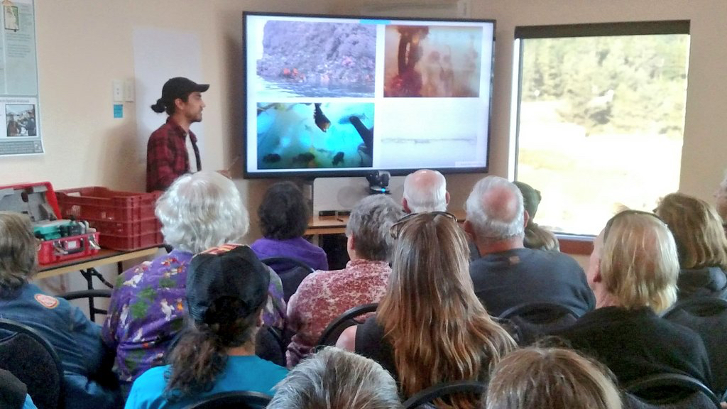
2018 team member Dylan presenting at the Port Orford community presentation. Source: T. Calvanese.
I think almost everyone in the scientific community would agree that outreach and engagement are important and that we should strive to interact frequently with the public to be transparent and build public trust, as well as to enable mutual learning. However, in my opinion, most scientists rarely put in the work needed to actually reach out to, and engage with, the community. Outreach and engagement have become buzzwords that are often thrown around, and with some hand-waving, can create the illusion that scientists are doing solid outreach and engagement work. For some, the words are probably even used interchangeably, which isn’t correct as they mean two different things.
Outreach and engagement should be thought of as occurring on two different ends of a spectrum. Outreach occurs in a one-way direction. Examples of outreach are public seminars delivered by a scientist (like Hatfield’s monthly Science on Tap) or fairs where the public is invited to come and talk to different scientific entities at their respective booths (like Hatfield’s annual Marine Science Day). Outreach is a way for scientists to disseminate their research to the public and often do not warrant the umbrella term engagement, as these “conversations” are not two-way. Engagement is collaborative and refers to intentional interactions where both sides (public and scientist) share and receive. It goes beyond a scientist telling the public about what they have been doing, but also requires the scientist to listen, absorb, and implement what the views from the ‘other side’ are.
2015 team tracking a whale on Graveyard Point above the port of Port Orford. Source: F. Sullivan.
Now that I have (hopefully) clarified the distinction between the two terms, I am going to shift the focus to specifically talk about the Port Orford project. Before I do, I would like to emphasize that I do not think our outreach and engagement is the be-all and end-all. There is definitely room for improvement and growth, but I do believe that we actively work hard to do both and to center these aspects within the project, rather than doing it as an afterthought to tick a box.
In talking about outreach and engagement, I have been using the words ‘public’ and ‘community’. I think these words conjure an image of a big group of people, an entire town, county, state or even nation. While this can be the case, it can also refer to smaller groups of people, even individuals. The outreach we conduct for the Port Orford project certainly occurs at the town-level. At the end of every field season, we give a community presentation where the field team and Leigh present new findings and give a recount of the field season. In the past, various teams have also given talks at the Humbug Mountain Campground and at Redfish Rocks Community Team events. These events, especially the community presentation, have been packed to the brim every year, which shows the community’s interest for the gray whales and our research. In fact, Tom Calvanese, the OSU Port Orford Field Station manager, has shared with me that now in early summer, Port Orford residents ask him when the ‘whale team’ is returning. I believe that our project has perhaps shifted the perception the local community has of scientists a little bit. Although in our first year or two of the project we may have been viewed as nosy outsiders, I feel that now we are almost honorary members within the community.
A packed room at the 2017 Port Orford community presentation. Photo: GEMM Lab.
Our outreach is not just isolated to one or two public talks per field season though. We have been close collaborators with South Coast Tours (SCT), an adventure tour company headed by Dave Lacey, since the start of the project. During the summer, SCT has almost daily kayak and fishing tours (this year, boat tours too!) out of Port Orford. The paddle routes of SCT and our kayak team will typically intersect in Tichenor’s Cove around mid-morning. When this happens, we form a little kayak fleet with the tour and research kayaks and our kayak team gives a short, informal talk about our research. We often pass around samples of zooplankton we just collected and answer questions that many of the paddlers have. These casual interactions are a highlight to the guests on SCT’s tours (Dave’s words, not mine) and they also provide an opportunity for the project’s interns to practice their science communication skills in a ‘low-stakes’ setting.
The nature of our engagement is more at the individual-level. Since the project’s conception in 2015, the team has been composed of some combination of 4-5 students, be it high school, undergraduate or graduate students. Aside from Florence Sullivan and myself as the GEMM Lab graduate student project leads, in total, we have had 16 students participate in the program, of which 4 were high school students (two from Port Orford’s Pacific High School and two from Astoria High School), 11 OSU and Lawrence University undergraduates, and 1 Duke University graduate student. This year we will be adding 3 more to the total tally (1 Pacific High School student, 1 OSU undergrad, and 1 graduate student from the Vrije Universiteit Brussel in Belgium). I am the first to admit that our yearly (and total) numbers of ‘impacted’ students is small. Limitations of funding and also general logistics of coordinating a large group of interns to participate in field work prevent us from having a larger cohort participate in the field season every summer. However, the impact on each of these students is huge.
The 2019 team with Dave Lacey who instructed our kayak paddle & safety course. Photo: L. Hildebrand.
If I had to pick one word to describe the 6-week Port Orford field season, it would be ‘intense’. The word is perfect because it can simultaneously describe something positive and negative, and the Port Orford field season definitely has elements of both. Both as a team and as individuals we experience incredible high points (an example being last year when we saw Port Orford’s favorite whale ‘Buttons’ breach multiple times on several different days), but we also have pretty low points (I’m thinking of a day in 2018 when two of my interns tried incredibly hard to get our GoPro stick dislodged from a rocky crevice for over 1-hour before radioing me to tell me they couldn’t retrieve it). These highs and lows occur on top of the team’s slowly depleting levels of energy as the field season goes on; with every day we get up at 5:30 am and we get a little more exhausted. The work requires a lot of brain power, a lot of muscle, and a lot of teamwork. Like I said, it’s intense and that’s coming from someone who had several years of marine mammal field work experience before running this project for the first time in 2018. The majority of the interns who have participated in our project have had no marine mammal field experience, some have had no field experience at all. It’s double, if not triple, intense for the interns!
I ask a lot of my interns. I am aware of that. It has been a steep learning curve for me since I took on the project in 2018. I’ve had to adjust my expectations and remember not to measure the performance of my interns against my own. I can always give 110% during the field season, even when I’m exhausted, because the stakes are high for me. After all, the data that is being collected feeds straight into my thesis. However, it took me a while to realize that the stakes, and therefore the motivation, aren’t the same for my interns as they are for me. And so, expecting them to perform at the same level I am, is unfair. I believe I have grown a lot since running that first field season. I have taken the feedback from interns to heart and tried to make adjustments accordingly. While those adjustments were hard because it ultimately meant making compromises that affected the amount of data collected, I recognize and respect the need to make those adjustments. I am incredibly grateful to all of the interns, including the ones that participated before my leadership of the project, who really gave it their all to collect the data that I now get to dig into and draw conclusions from.
2016 interns Kelli and Catherine paddling to a kayak sampling station. Photo: F. Sullivan.
But, as I said before, engagement is not one-sided, and I am not the only one who benefits from having interns participate in the project. The interns themselves learn a wealth of skills that are valuable for the future. Some of these skills are very STEM (Science, Technology, Engineering & Mathematics) specific (e.g. identifying zooplankton with a microscope, tracking whales with a theodolite), but a lot of them are transferrable to non-STEM futures (e.g. attention to detail and concentration required for identifying zooplankton, team work, effective communication). Our reach may be small with this project but the impact that participating in our internship has on each intern is a big one. Three of our four high school interns have gone on to start college. One plans to major in Marine Studies (in part a result of participating in this internship) while another decided to go to college to study Biology because of this internship. Several of the undergraduate students that participated in the 2015, 2016, 2017 & 2018 field seasons have gone on to start Master’s degrees at graduate schools around the country (3 of which have already graduated from their programs). A 2015 intern now teaches middle school in Washington and a 2016 intern is working with Oceans Initiative on their southern resident killer whale project this summer. Leigh, Florence and I have written many letters of recommendations for our interns, and these letters were not written out of duty, but out of conviction.
I love working closely with students and watching them grow. For the last two years, my proudest moment has always been watching my interns present our research at the annual community presentation we give at the end of the field season in Port Orford. No matter the amount of lows and struggles I experienced throughout the season, I watch my interns and my face almost hurts because of the huge smile on my face. The interns truly undergo a transformation where at the start of the season they are shy or feel inadequate and awkward when talking to the public about gray whales and the methods we employ to study them. But on that final day, there is so much confidence and eloquence with which the interns talk about their internship, that they are oftentimes even comfortable enough to crack jokes and share personal stories with the audience. As I said before, engagement of this nature is hard to measure and put a number on. Our statistic (engaging with 16 students) makes it sound like a small impact, but when you dig into what these engagements have meant for each student, the impact is enormous.
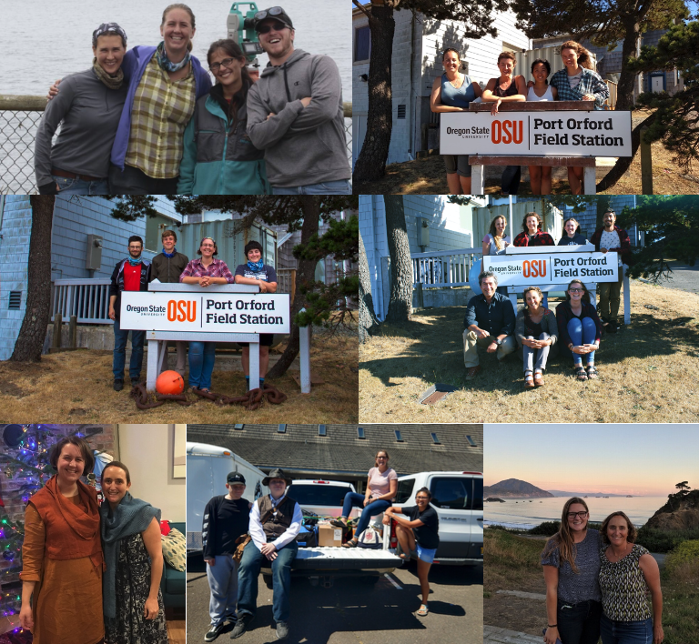
All of the past PO gray whale ecology teams, from left to right: 2015 (Sarah, Florence, Cricket, Justin), 2016 (Florence, Kelli, Catherine, Cathryn), 2017 (Nathan, Quince, Florence, Morgan), 2018 (Haley, Robyn, Hayleigh, Dylan, Lisa), and 2019 (Anthony, Donovan, Lisa, Mia). Bottom left: Florence and Leigh; bottom right: Lisa and Leigh.
I treasure my 6 weeks in Port Orford. Even though they are intense and there are new challenges every year, they bring me a lot of happiness. And it’s only in part because I get to see gray whales and kayak on an (almost) daily basis. A large part is because of the bonds I have formed and continue to cultivate with Port Orford locals, the leaps and bounds I know the interns will make, and the fact that the gray whales, completely unknowingly, bring together a small group of students and a community every year.
If you feel like taking a trip down memory lane, below are the links of the blogs written by previous PO interns:
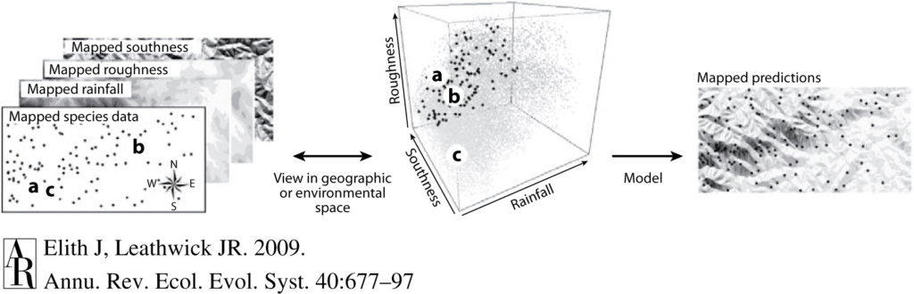
Recently, I had the opportunity to attend the International Statistical Ecology Conference (ISEC), a biennial meeting of researchers at the interface of ecology and statistics. I am a marine ecologist, fascinated by the interactions between animals and the dynamic ocean environment they inhabit. If you had asked me five years ago whether I thought I would ever consider myself a statistician or a computer programmer, my answer would certainly have been “no”. Now, I find myself studying the ecology of blue whales in New Zealand using a variety of data streams and methodologies, but a central theme for my dissertation is species distribution modeling. Species distribution models (SDMs) are mathematical algorithms that correlate observations of a species with environmental conditions at their observed locations to gain ecological insight and predict spatial distributions of the species (Fig. 1; Elith and Leathwick 2009). I still can’t say I would identify as a statistician, but I have a growing appreciation for the role of statistics to gain inference in ecology.
Figure 1. A schematic of a species distribution model (SDM) illustrating how the relationship between mapped species and environmental data (left) is compared to describe “environmental space” (center), and then map predictions from a model using only environmental predictors (right). Note that inter-site distances in geographic space might be quite different from those in environmental space—a and c are close geographically, but not environmentally. The patterning in the predictions reflects the spatial autocorrelation of the environmental predictors. Figure reproduced from Elith and Leathwick (2009).
Before I continue, let’s take a look at just a few definitions from Merriam-Webster’s dictionary:
Statistics: a branch of mathematics dealing with the collection, analysis, interpretation, and presentation of masses of numerical data
Ecology: a branch of science concerned with the interrelationship of organisms and their environments
Inference: a conclusion or opinion that is formed because of known facts or evidence
Ecological data are notoriously noisy, messy, and complex. Statistical tests are meant to help us understand whether a pattern in the data is different from what we would expect through random chance. When we study how organisms interact with one another and their environment, it is impossible to completely capture all elements of the ecosystem. Therefore, ecology is a field ripe with challenges for statisticians. How do we quantify a meaningful biological signal amidst all the noise? How can we gain inference from ecological data to enhance knowledge, and how can we use that knowledge to make informed predictions? Marine mammals are notoriously difficult to study. They inhabit an environment that is relatively inaccessible and inhospitable to humans, they occur in low numbers, they are highly mobile, and they are rarely visible. All ecological data are difficult and noisy and riddled with small sample sizes, but counting trees presents fewer logistical challenges than counting moving whales in an ever-changing open-ocean setting. Therefore, new methodologies in areas like species distribution modeling are often developed using large, terrestrial datasets and eventually migrate to applications in the marine environment (Robinson et al. 2011).
Many presentations I attended at the conference were geared toward moving beyond correlative SDMs. SDMs were developed to correlate species occurrence patterns with features of the environment they inhabit (e.g. temperature, precipitation, terrain, etc.). However, those relationships do not actually explain the underlying mechanism of why a species is more likely to occur in one environment compared to another. Therefore, ecological statisticians are now using additional information and modeling approaches within SDMs to incorporate information such as species co-occurrence patterns, population demographic information, and physiological constraints. Building SDMs to include such process-explicit information allows us to make steps toward understanding not just when and where a species occurs, but why.
Machine learning is an area that continues to advance and open doors to new applications in ecology. Machine learning approaches differ fundamentally from classical statistics. In statistics, we formulate a hypothesis, select the appropriate model to test that hypothesis (for example, linear regression), then test how well the data fit the model (“Is the relationship linear?”), and test the strength of that inference (“Is the linear pattern different from what we would expect due to random chance?”). Machine learning, on the other hand, does not use a predetermined notion of relationships between variables. Rather, it tries to create an algorithm that fits the patterns in the data. Statistics asks how well the data fit a model, and machine learning asks how well a model fits the data.
Machine learning approaches allow for very complex relationships to be included in models and can be excellent for making predictions. However, sometimes the relationships fitted by a machine learning algorithm are so complex that it is not possible to infer any ecological meaning from them. As one ISEC presenter put it, in machine learning “the computer learns but the scientist does not”. The most important thing when selecting your methodology is to remember your question and your goal. Do you want to understand the mechanism of why an animal is where it is? Or do you not need to understand the driver, but rather want to make the best predictions of where an animal will be? In my case, the answer to that question differs from one of my PhD chapters to the next. We want to understand the functional relationships between oceanography, krill availability, and blue whale distribution (Barlow et al. 2020), and subsequently we want to develop forecasting models that can reliably predict blue whale distribution to inform conservation efforts (Fig. 2).
Figure 2. An example predictive map of where we expect blue whales to be distributed based on environmental conditions. Warmer colors represent areas with a higher probability of blue whale occurrence, and the blue crosses represent locations where blue whales were observed.
ISEC was an excellent opportunity for me to break out of my usual marine mammal-centered bubble and get a taste of what is happening on the leading edge of statistical ecology. I learned about the latest approaches and innovations in species distribution modeling, and in the process I also learned about trees, koalas, birds, and many other organisms from around the world. A fun bonus of attending a methods-focused conference is learning about completely new study species and systems. There are many ways of approaching an ecological question, gaining inference, and making predictions. I look forward to incorporating the knowledge I gained through ISEC into my own research, both in my doctoral work and in applications of new methods to future research projects.
Figure 3. The virtual conference photo of all who attended the biennial International Statistical Ecology Conference. Thank you to the organizers, who made it a truly excellent and engaging conference experience!
References
Barlow, D.R., Bernard, K.S., Escobar-Flores, P., Palacios, D.M., and Torres, L.G. 2020. Links in the trophic chain: Modeling functional relationships between in situ oceanography, krill, and blue whale distribution under different oceanographic regimes. Mar. Ecol. Prog. Ser. doi:https://doi.org/10.3354/meps13339.
Elith, J., and Leathwick, J.R. 2009. Species Distribution Models: Ecological Explanation and Prediction Across Space and Time. Annu. Rev. Ecol. Evol. Syst. 40(1): 677–697. doi:10.1146/annurev.ecolsys.110308.120159.
Robinson, L.M., Elith, J., Hobday, A.J., Pearson, R.G., Kendall, B.E., Possingham, H.P., and Richardson, A.J. 2011. Pushing the limits in marine species distribution modelling: Lessons from the land present challenges and opportunities. doi:10.1111/j.1466-8238.2010.00636.x.
By Hunter Warick, Research Technician, Geospatial Ecology of Marine Megafauna Lab, Marine Mammal Institute
When monitoring the health of a capital breeding species, such as whales that store energy to support reproduction costs, it is important to understand what processes and factors drive the status of their body condition. Information gained will allow for better insight into their cost of reproduction and overall life history strategies.
For the past four years the GEMM Lab has utilized the perspective that Unoccupied Aerial Systems (UAS; or ‘drones’) provide for observations of marine mammals. This aerial perspective has documented gray whale behavior such as jaw snapping, drooling mud, and headstands, all of which shows or suggest foraging (Torres et al. 2018). However, UAS is limited to a bird’s eye view, allowing us to see WHAT whales are doing, but limited information about the reasons WHY. To overcome this hurdle, Leigh Torres and team have equipped their marine mammal research utility belts with the use of GoPro cameras. They developed a technique known as the “GoPro drop” where a GoPro camera mounted to a weighted pole is lowered off the side of the research vessel in waters < 20 m deep via a line to record video data. This technique allows the team to obtain fine-scale habitat and prey variation information, like what the whale experiences. Along with the context provided by the UAS, this dual camera perspective allows for deeper insight into gray whale foraging strategies and efficiency. Torres’s GoPro data analysis protocol examines kelp density, kelp health, benthic substrate, rock fish density, and mysid density. These characteristics are graded along a scale (Figure 1), allowing for relative comparisons of habitat and prey availability between where whales spend time and forage. These GoPro drops will also help create a fine-scale benthic habitat map of the Newport field area. So, why are these data on gray whale habitat and prey important to understand?
Figure 1. The top row shows varying degrees of mysid density (low to high, left to right). Middle row illustrates different types of substrate you might encounter (reef, sandy, boulders; left to right). Bottom row shows the different levels of kelp health (poor, medium, good).
The foraging grounds are the first step in the life history domino chain reaction for many rorqual whales; if this step doesn’t go off cleanly then everything else fails to fall into place. Gray whales partake on a 15,000-20,000 km (round trip) migration, which is the longest of any known mammal (Swartz 1986). During this migration, whales spend around three months fasting in their breeding grounds (Highsmith & Coyle 1992), living only off the energy stores that they accumulated in their feeding grounds (Næss et al. 1998). These extreme conditions of existence for gray whales drive the need to be a successful forager and is why it is so crucial for them to forage in high prey density areas (Newell, C. 2009).
Mysids are a critical part of the gray whale diet in Oregon waters (Newell, C. 2009; Sullivan, F. 2017) and mysids have strong predator-prey relationships with both top-down and bottom-up control (Dunham & Duffus 2001; Newell & Cowles 2006). This unique tie illustrates the great dependency that gray whales have on mysids, further showing the benefit to looking at the density of mysids where gray whales are seen foraging. The quality of mysids may also be as important as quantity; with higher water temperatures resulting in lower lipid content in mysids (Mauchline 1980), suggesting density might not be the only factor for determining efficient whale foraging. The overall goal of gray whales on their foraging grounds is to get as fat as possible in order to reproduce as often as possible. But, this isn’t always as easy as it sounds. Gray whales typically have a two-year breeding interval but can be anywhere from 1-4 years (Blokhin 1984). The longer time it takes to build up adequate energy stores to support reproduction costs, the longer it will take to breed successfully. Building back up these energy stores can prove to be difficult, especially for lactating females (Figure 2).
Figure 2. Comparison of body condition between a lactating female gray whale on the feeding grounds in Newport, Oregon, 2020 (GEMM Lab, OSU; NOAA/NMFS permit # 21678) and a pregnant female gray whale on the breeding grounds in San Ignacio Lagoon, 2019 (provided by Laguna San Ignacio Ecosystem Program). Photographer Hunter Warick. Note the very different body shapes: thin lactating female relative to the rotund pregnant female.
Being able to track the health and behavior of gray whales on an individual level, including comparisons between variation in body condition, foraging behavior, and fine scale information on benthic communities gained through the use of GoPros, can provide a better understanding of the driving factors and impacts on their health and population trends (Figure 3).
Figure 3. A compilation of video clips captured by the GEMM Lab during their research on gray whale ecology and physiology off Newport, Oregon using Unoccupied Aerial Systems (UAS, or “drones”) and GoPro cameras. UAS are used to observe gray whale behavior and conduct photogrammetry assessment of body condition. GoPro camera drops assess the benthic habitat and prey density across the study region, with a couple chance encounters of whales. Research is conducted under NOAA/NMFS permit # 21678.
Clara Bird, Masters Student, OSU Department of Fisheries and Wildlife, Geospatial Ecology of Marine Megafauna Lab
A big part of graduate school involves extensive reading to learn about the previous research conducted in the field you are joining and the embedded foundational theories. A firm understanding of this background literature is needed in order to establish where your research fits. Science is a constructive process; to advance our disciplines we must recognize and build upon previous work. Hence, I’ve been reading up on the central topic of my thesis: behavioral ecology. It is equally important to study the methods used in these studies as to understand the findings. As discussed in a previous blog, ethograms are a central component of the methodology for studying behavior. Ethograms are lists of defined behaviors that help us properly and consistently collect data in a standardized approach. It is especially important in a project that spans years to know that the data collected at the beginning was collected in the same way as the data collected at the end of the project.
While ethograms and standardized methods are commonly used within a study, I’ve noticed from reading through studies on cetaceans, a lack of standardization across studies. Not all behaviors that are named the same way have matching definitions, and not all behaviors with similar definitions have matching names. Of all the behaviors, “milling” may be the least standardized.
While milling is not in our ethogram (Leigh believes this term is a “cheat” for when behavior is actually “unknown”), we occasionally use “milling” in the field to describe when the gray whales are swimming around in an area, not foraging, but not in any other primary behavior state (travel, social, or rest). Sometimes we use when we think the whale may be searching, but we aren’t 100% sure yet. A recent conversation during a lab meeting on the confusing nature of the term “milling” inspired me to dig into the literature for this blog. I searched through the papers I’ve saved for my literature review and found 18 papers that used the term milling. It was fascinating to read how variably the term has been defined and used.
When milling was defined in these papers, it was most commonly described as numerous directional changes in movement within a restricted area 1–8. Milling often co-occurred with other behavior states. Five of these eight studies described milling as co-occurring with foraging behavior 3–6,8. In one case, milling was associated with foraging and slow movement 8. While another study described milling as passive, slow, nondirectional movement 9.
Eight studies used the term milling without defining the behavior 10–17. Of these, five described milling as being associated with other behavior states. Three studies described milling as co-occurring with foraging 10,14,16, one said that it co-occurred with social behavior 13, and another described milling as being associated with resting/slow movement 12.
In addition to this variety of definitions and behavior associations, there were also inconsistencies with the placement of “milling” within ethograms. In nine studies, milling was listed as a primary state 1,2,4,7–9,15,17,18. But, in two studies that mentioned milling and used an ethogram, milling was not included in the ethogram 6,14.
Diving into the associations between milling and foraging reveal how varied the use of milling has been within the cetacean literature. For example, two studies simply described milling as occurring near foraging in time 10,16. While another two studies explained that milling was applied in situations where there was evidence of feeding without feeding being directly observed 8,14. Bobkov et al. (2019) described milling as occurring between feeding cycles along with breathing. Lastly, two studies describe milling as a behavior within the foraging primary state 3,5, while another study described feeding as a behavior within milling 4.
It’s all rather confusing, huh? Across these studies, milling has been defined, mentioned without being defined, included in ethograms as a primary state, included in ethograms as a sub-behavior, and excluded from ethograms. Milling has also been associated with multiple primary behavior states (foraging, resting, and socializing). It has been described as both passive 9 and slow 12, and strong 16 and active 5.
It appears that milling is often used to describe behaviors that the observer cannot distinctly classify or describe its function. I have also struggled to define these times when a whale is in between behavior states; I often end up calling it “just being a whale”, which includes time spent breathing at the surface, or just swimming around.
As I’ve said above, Leigh thinks that this term is a “cheat” for when a behavior is actually “unknown”. I think we have trouble equating “milling” with “unknown” because it seems like “unknown” should refer to a behavior where we can’t quite tell what the whale is doing. However, during milling, we can see that the whale is swimming at the surface. But here’s the thing, while we can see what the whale is doing, the function of the behavior is still unknown. Instead of using an indistinct term, we should use a term that better describes the behavior. If it’s swimming at the surface, name the behavior “swimming at the surface”. If we can’t tell what the whale is doing because we can’t quite see what it’s doing, then name the behavior “unknown-partially visible”. Instead of using vague terminology, we should use clear names for behaviors and embrace using the term “unknown”.
I am most certainly not criticizing these studies as they all provided valuable contributions and interesting results. The studies that asked questions about behavioral ecology defined milling. The term was mentioned without being defined in studies focused on other topics. So, defining behaviors mentioned was less important.
With this exploration into the use of “milling” in studies, I am not implying that all behavioral ecologists need to agree on the use of the same behavior terms. However, I have learned clear definitions are critical. This lesson is also important outside of behavioral ecology. Different labs, and different people, use different terms for the same things. As I dig into my thesis, I am keeping a list of terminology I use and how I define those terms, because as I learn more, my terminology evolves and changes. For example, at the beginning of my thesis I used “sub-behavior” to refer to behaviors within the primary state categories. But, now after chatting with Leigh and learning more, I’ve decided to use the term “tactic” instead as these are often processes or events that contribute to the broader behavior state. My running list of terminology helps me remember what I meant when I used a certain word, so that when I read my notes from three months ago, I can know what I meant. Digging into the literature for this blog reminded me of the importance of clearly defining all terminology and never assuming that everyone uses the same term in the same way.
Check out these videos to see some of the behaviors we observe:
References
1. Mallonee, J. S. Behaviour of gray whales (Eschrichtius robustus) summering off the northern California coast, from Patrick’s Point to Crescent City. Can. J. Zool.69, 681–690 (1991).
2. Clarke, J. T., Moore, S. E. & Ljungblad, D. K. Observations on gray whale (Eschrichtius robustus) utilization patterns in the northeastern Chukchi Sea. Can. J. Zool67, (1988).
3. Ingram, S. N., Walshe, L., Johnston, D. & Rogan, E. Habitat partitioning and the influence of benthic topography and oceanography on the distribution of fin and minke whales in the Bay of Fundy, Canada. J. Mar. Biol. Assoc. United Kingdom87, 149–156 (2007).
4. Lomac-MacNair, K. & Smultea, M. A. Blue Whale (Balaenoptera musculus) Behavior and Group Dynamics as Observed from an Aircraft off Southern California. Anim. Behav. Cogn.3, 1–21 (2016).
5. Lusseau, D., Bain, D. E., Williams, R. & Smith, J. C. Vessel traffic disrupts the foraging behavior of southern resident killer whales Orcinus orca. Endanger. Species Res.6, 211–221 (2009).
6. Bobkov, A. V., Vladimirov, V. A. & Vertyankin, V. V. Some features of the bottom activity of gray whales (Eschrichtius robustus) off the northeastern coast of Sakhalin Island. 1, 46–58 (2019).
7. Howe, M. et al. Beluga, Delphinapterus leucas, ethogram: A tool for cook inlet beluga conservation? Mar. Fish. Rev.77, 32–40 (2015).
8. Clarke, J. T., Christman, C. L., Brower, A. A. & Ferguson, M. C. Distribution and Relative Abundance of Marine Mammals in the northeastern Chukchi and western Beaufort Seas, 2012. Annu. Report, OCS Study BOEM117, 96349–98115 (2013).
9. Barendse, J. & Best, P. B. Shore-based observations of seasonality, movements, and group behavior of southern right whales in a nonnursery area on the South African west coast. Mar. Mammal Sci.30, 1358–1382 (2014).
10. Le Boeuf, B. J., M., H. P.-C., R., J. U. & U., B. R. M. and F. O. High gray whale mortality and low recruitment in 1999: Potential causes and implications. (Eschrichtius robustus). J. Cetacean Res. Manag.2, 85–99 (2000).
11. Calambokidis, J. et al. Abundance, range and movements of a feeding aggregation of gray whales (Eschrictius robustus) from California to southeastern Alaska in 1998. J. Cetacean Res. Manag.4, 267–276 (2002).
12. Harvey, J. T. & Mate, B. R. Dive Characteristics and Movements of Radio-Tagged Gray Whales in San Ignacio Lagoon, Baja California Sur, Mexico. in The Gray Whale: Eschrichtius Robustus (eds. Jones, M. Lou, Folkens, P. A., Leatherwood, S. & Swartz, S. L.) 561–575 (Academic Press, 1984).
13. Lagerquist, B. A. et al. Feeding home ranges of pacific coast feeding group gray whales. J. Wildl. Manage.83, 925–937 (2019).
14. Barrett-Lennard, L. G., Matkin, C. O., Durban, J. W., Saulitis, E. L. & Ellifrit, D. Predation on gray whales and prolonged feeding on submerged carcasses by transient killer whales at Unimak Island, Alaska. Mar. Ecol. Prog. Ser.421, 229–241 (2011).
15. Luksenburg, J. A. Prevalence of External Injuries in Small Cetaceans in Aruban Waters, Southern Caribbean. PLoS One9, e88988 (2014).
16. Findlay, K. P. et al. Humpback whale “super-groups” – A novel low-latitude feeding behaviour of Southern Hemisphere humpback whales (Megaptera novaeangliae) in the Benguela Upwelling System. PLoS One12, e0172002 (2017).
17. Villegas-Amtmann, S., Schwarz, L. K., Gailey, G., Sychenko, O. & Costa, D. P. East or west: The energetic cost of being a gray whale and the consequence of losing energy to disturbance. Endanger. Species Res.34, 167–183 (2017).
18. Brower, A. A., Ferguson, M. C., Schonberg, S. V., Jewett, S. C. & Clarke, J. T. Gray whale distribution relative to benthic invertebrate biomass and abundance: Northeastern Chukchi Sea 2009–2012. Deep. Res. Part II Top. Stud. Oceanogr.144, 156–174 (2017).
By Alejandro Fernandez Ajo, PhD student at the Department of Biology, Northern Arizona University, Visiting scientist in the GEMM Lab working on the gray whale physiology and ecology project
Whales are among the most amazing and enigmatic animals in the world. Whales are not only fascinating, they are also biologically special. Due to their key ecological role and unique biological traits (i.e., their large body size, long lifespans, and sizable home ranges), whales are extremely important in helping sustain the entire marine ecosystem.
Working towards the conservation of marine megafauna, and large charismatic animals in general, is often seen as a mere benevolent effort that conservationist groups, individuals, and governments do on behalf of the individual species. However, mounting evidence demonstrates that restoring populations of marine megafauna, including large whales, can help buffer marine ecosystems from destabilizing stresses like human driven CO2 emissions and global change due to their ability to sequester carbon in their bodies (Pershing et al. 2010). Furthermore, whales can enhance primary production in the ocean through their high consumption and defecation rates, which ultimately provides nutrients to the ecosystem and improves fishery yields (Roman-McCarthy, 2010; Morissette et al. 2012).
Relationships between humans and whales have a long history, however, these relationships have changed. For centuries, whales were valued in terms of the number of oil barrels they could yield, and the quality of their baleen and meat. In the North Atlantic, whaling started as early as 1000 AD with “shore whaling” of North Atlantic right whales by Basque whalers. This whaling was initially limited to the mother and calve pairs that were easy to target due to their coastal habits and the fact that calves are more vulnerable and slower (Reeves-Smith, 2006). Once the calving populations of near-shore waters off Europe were depleted, offshore whaling began developing. Whalers of multiple nations (including USA, British, French, Norwegian, Portuguese, and Dutch, among others), targeted whales around the world, mainly impacting the gray whale populations, and all three right whale species along with the related bowhead whale. Later, throughout the phase of modern whaling using industrialized methods, the main target species consisted of the blue, fin, humpback, minke, sei and sperm whale (Schneider- Pearce, 2004).
By the early twentieth century, many of the world´s whale populations where reduced to a small fraction of their historical numbers, and although pre-whaling abundance of whale stocks is a subject of debate, recent studies estimate that at least the 66%, and perhaps as high as 90% for some whale species and populations (Branch-Williams 2006; Christensen, 2006), where taken during this period. This systematic and serial depletion of whale papulations reduced the biomass and abundance of great whales around the world, which has likely altered the structure and function of the oceans (Balance et al. 2006; Roman et al. 2014; Croll, et al. 2006).
After centuries of unregulated whale hunting, commercial whaling was banned in the mid-twentieth century. This ban was the result of multiple factors including reduced whale stocks below the point where commercial whaling would be profitable, and a fortunate shift in public perception of whales and the emergence of conservation initiatives (Schneider- Pearce, 2004). Since this moratorium on whaling, several whale populations have recovered around the world, and some populations that were listed as endangered have been delisted (i.e., the Eastern North Pacific gray whale) and some populations are estimated to have re-bounced to their pre-whaling abundance.
Although, the recovery of some populations has motivate some communities or nations to obtain or extend their whaling quotas (see Blog Post by Lisa Hildebrand), it is important to acknowledge that the management of whale populations is arguably one of the most complicated tasks, and is distinguished from management of normal fisheries due to various biological aspects. Whales are long living mammals with slow reproduction rates, and on average a whale can only produce a calf every two or three years. Hence, the gross addition to the stock rarely would exceed 25% of the number of adults (Schneider- Pearce, 2004), which is a much lower recovery rate that any fish stock. Also, whales usually reach their age of sexual maturity at 6-10 years old, and for many species there are several uncertainties about their biology and natural history that make estimations of population abundance and growth rate even harder to estimate.
Fig 1: Human relationship with whales has changed through history. Once valued for their meat and oil, now they are a natural attraction that amaze and attract crowds to whale watching destinations all over the globe. Photo: Stephen Johnson, Península Valdés-Argentina.
Moreover, while today´s whales are generally not killed directly by hunting, they are exposed to a variety of other increasing human stressors (e.g., entanglement in fishing gear, vessel strikes, shipping noise, and climate change). Thus, scientists must develop novel tools to overcome the challenges of studying whales and distinguish the relative importance of the different impacts to help guide conservation actions that improve the recovery and restoration of whale stocks (Hunt et al. in press). With the restoration of great whale populations, we can expect positive changes in the structure and function of the world’s oceans (Chami et al. 2019; Roman et al. 2010).
So, why it is worth keeping whales healthy?
Whales facilitate the transfer of nutrients by (1) releasing nutrient-rich fecal plumes near the surface after they have feed at depth and (2) by moving nutrients from highly productive, polar and subpolar latitude feeding areas to the low latitude calving areas (Roman et al. 2010). In this way, whales help increase the productivity of phytoplankton that in turn support zooplankton production, and thus have a bottom up effect on the productivity of many species including fish, birds, and marine mammals, including whales. These fertilization events can also facilitate mitigation of the negative impacts of climate change. The amount of iron contained in the whales’ feces can be 10 million times greater than the level of iron in the marine environment, triggering important phytoplankton blooms, which in turn sequester thousands of tons of carbon from, and release oxygen to, the atmosphere annually (Roman et al. 2016; Smith et al. 2013; Willis, 2007). Furthermore, when whales die, their massive bodies fall to the seafloor, making them the largest and most nutritious source of food waste, which is capable of sustaining a succession of macro-fauna assemblages for several decades, including some invertebrate species that are endemic to whale carcasses (Smith et al. 2015).
Figure 2. The figure shows a conceptual model of the “whale pump”. From Roman-McCarthy, 2010.
Despite the several environmental services that whales provide, and the positive impact on local economies that depend on whale watching tourism, which has been valued in millions of dollars per year (Hoyt E., 2001), the return of whales and other marine mammals has often been implicated in declines in fish populations, resulting in conflicts with human fisheries (Lavigne, D.M. 2003). Yet there is insufficient direct evidence for such competition (Morissette et al. 2010). Indeed, there is evidence of the contrary: In ecosystem models where whale abundances are reduced, fish stocks show significant decreases, and in some cases the presence of whales in these models result in improved fishery yields. Consistent with these findings, several models have shown that alterations in marine ecosystems resulting from the removal of whales and other marine mammals do not lead to increases in human fishery yields (Morissette et al. 2010; 2012). Although the environmental services and benefits provided by great whales, which potentially includes the enhancement of fisheries yields, and enhancement on ocean oxygen production and capturing carbon, are evident and make a strong argument for improved whale conservation, it is overwhelming how little we know about many aspects of their lives, their biology, and particularly their physiology.
Figure 3: Whales are the most fascinating animals in the world, but they are not only amazing animals. They are also extremely important in sustaining the entire marine ecosystem. Photo: Alejandro Fernández Ajó -Instituto de Conservación de ballenas.
This lack of knowledge is because whales are really hard to study. For many years research was limited to the observation of the brief surfacing of the whales, yet most of their lives occurs beneath the surface and were completely unknown. Fortunately, new technologies and the creativity of whale researchers are helping us to better understand many aspects of their lives that were cryptic to us even a decade ago. I am committed to filling some of these knowledge gaps. My research examines how different environmental and anthropogenic impacts affect whale health, and particularly how these impacts may relate to cases of large whale mortalities and declines in whale populations. I am applying novel methods in conservation physiology for measuring hormone levels that promise to improve our understanding of the relationship between different (extrinsic and intrinsic) stressors and the physiological response of whales. Ultimately, this research will help address important conservation questions, such as the causes of unusual whale mortality events and declines in whale populations.
References:
Ballance LT, Pitman RL, Hewitt R, et al. 2006. The removal of large whales from the Southern Ocean: evidence for long-term ecosystem effects. In: Estes JA, DeMaster DP, Doak DF, et al. (Eds). Whales, whaling and ocean ecosystems. Berkeley, CA: University of California Press.
Branch TA and Williams TM. 2006. Legacy of industrial whaling. In: Estes JA, DeMaster DP, Doak DF, et al. (Eds). Whales, whaling and ocean ecosystems. Berkeley, CA: University of California Press.
Chami, R. Cosimano, T. Fullenkamp, C. & Oztosun, S. (2019). Nature’s solution to climate change. Finance & Development, 56(4).
Christensen LB. 2006. Marine mammal populations: reconstructing historical abundances at the global scale. Vancouver, Canada: University of British Columbia.
Croll DA, Kudela R, Tershy BR (2006) Ecosystem impact of the decline of large whales in the North Pacific. In: Estes JA, DeMaster DP, Doak DF, Williams TM, BrownellJr RL, editors. Whales, Whaling, and Ocean Ecosystems. Berkeley: University of California Press. pp. 202–214.
Hoyt, E. 2001. Whale Watching 2001: Worldwide Tourism Numbers, Expenditures and Expanding Socioeconomic Benefits
Hunt, K.E., Fernández Ajó, A. Lowe, C. Burgess, E.A. Buck, C.L. In press. A tale of two whales: putting physiological tools to work for North Atlantic and southern right whales. In: “Conservation Physiology: Integrating Physiology Into Animal Conservation And Management”, ch. 12. Eds. Madliger CL, Franklin CE, Love OP, Cooke SJ. Oxford University press: Oxford, UK.
Lavigne, D.M. 2003. Marine mammals and fisheries: the role of science in the culling debate. In: Gales N, Hindell M, and Kirkwood R (Eds). Marine mammals: fisheries, tourism, and management issues. Melbourne, Australia: CSIRO.
Morissette L, Christensen V, and Pauly D. 2012. Marine mammal impacts in exploited ecosystems: would large scale culling benefit fisheries? PLoS ONE 7: e43966.
Morissette L, Kaschner K, and Gerber LR. 2010. “Whales eat fish”? Demystifying the myth in the Caribbean marine ecosystem. Fish Fish 11: 388–404.
Pershing AJ, Christensen LB, Record NR, Sherwood GD, Stetson PB (2010) The impact of whaling on the ocean carbon cycle: Why bigger was better. PLoS ONE 5(8): e12444.
Reeves, R. and Smith, T. (2006). A taxonomy of world whaling. In DeMaster, D. P., Doak, D. F., Williams, T. M., and Brownell Jr., R. L., eds. Whales, Whaling, and Ocean Ecosystems. University of California Press, Berkeley, CA.
Roman, J. Altman I, Dunphy-Daly MM, et al. 2013. The Marine Mammal Protection Act at 40: status, recovery, and future of US marine mammals. Ann NY Acad Sci; doi:10.1111/nyas.12040.
Roman, J. and McCarthy, J.J. 2010. The whale pump: marine mammals enhance primary productivity in a coastal basin. PLoS ONE. 5(10): e13255.
Roman, J. Estes, J.A. Morissette, L. Smith, C. Costa, D. McCarthy, J. Nation, J.B. Nicol, S. Pershing, A.and Smetacek, V. 2014. Whales as marine ecosystem engineers. Frontiers in Ecology and the Environment. 12(7). 377-385.
Roman, J. Nevins, J. Altabet, M. Koopman, H. and McCarthy, J. 2016. Endangered right whales enhance primary productivity in the Bay of Fundy. PLoS ONE. 11(6): e0156553.
Schneider, V. Pearce, D. What saved the whales? An economic analysis of 20th century whaling. Biodiversity and Conservation 13, 543–562 (2004). https://doi org.libproxy.nau.edu/10.1023/B:BIOC.0000009489.08502.1
Smith LV, McMinn A, Martin A, et al. 2013. Preliminary investigation into the stimulation of phyto- plankton photophysiology and growth by whale faeces. J Exp Mar Biol Ecol 446: 1–9.
Smith, C.R. Glover, A.G. Treude, T. Higgs, N.D. and Amon, D.J. 2015. Whale-fall ecosystems: Recent insights into ecology, paleoecology, and evolution. Annu. Rev. Marine. Sci. 7:571-596.
Willis, J. 2007. Could whales have maintained a high abundance of krill? Evol Ecol Res 9: 651–662.