I always have a small crisis before heading into the field, whether for a daytrip or a several-month stint. I’m always dying to go – up until the moment when it is actually time to leave, and I decide I’d rather stay home, keep working on whatever has my current focus, and not break my comfortable little routine.
Preparing to leave on the most recent Northern California Current (NCC) cruise was no different. And just as always, a few days into the cruise, I forgot about the rest of my life and normal routines, and became totally immersed in the world of the ship and the places we went. I learned an exponential amount while away. Being physically in the ecosystem that I’m studying immediately had me asking more, and better, questions to explore at sea and also bring back to land.
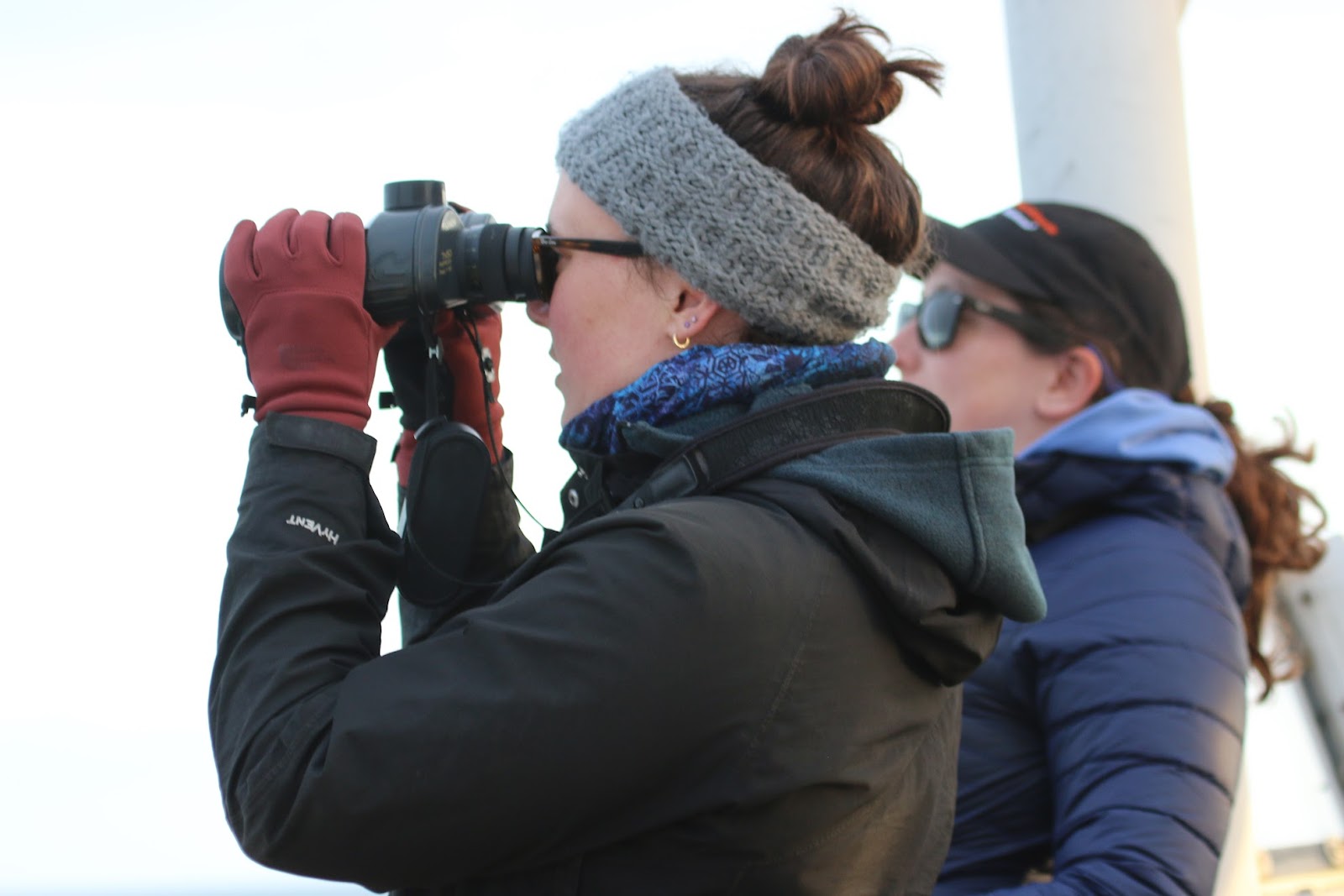
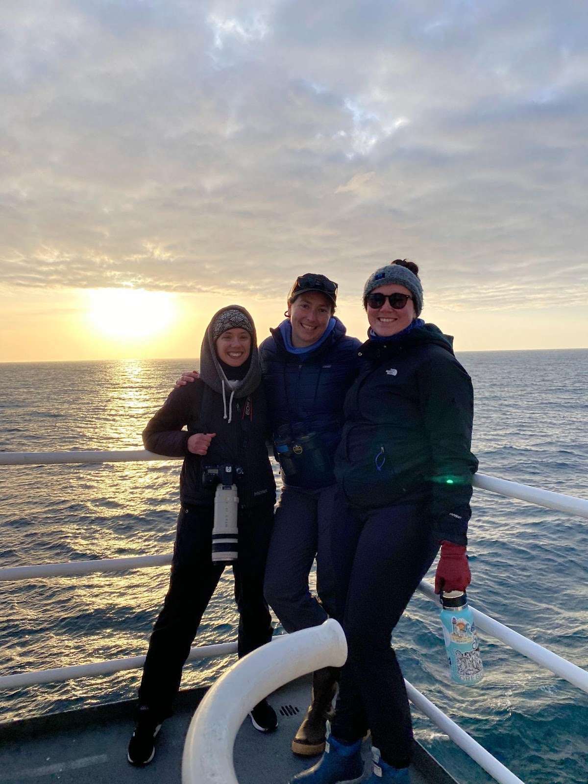
Many of these questions and realizations centered on predator-prey relationships between krill and whales at fine spatial scales. We know that distributions of prey species are a big factor in structuring whale distributions in the ocean, and one of our goals on this cruise was to observe these relationships more closely. The cruise offered an incredible opportunity to experience these relationships in real time: while my labmates Dawn and Clara were up on the flying bridge looking for whales, I was down in the acoustics lab, watching incoming echosounder data in order to identify krill aggregations.
From left, Clara and Dawn survey for marine mammals on the flying bridge.
We used radios to stay in touch with what we were each seeing in real time, and learned quickly that we tended to spot whales and krill almost simultaneously. Experiencing this coherence between predator and prey distributions felt like a physical manifestation of my PhD. It also affirmed my faith in one of our most basic modeling assumptions: that the backscatter signals captured in our active acoustic data are representative of the preyscape that nearby whales are experiencing.
Being at sea with my labmates also catalyzed an incredible synthesis of our different types of knowledge. Because of the way that I think about whale distributions, I usually just focus on whether a certain type of whale is present or not while surveying. But Clara, with her focus on cetacean behavior, thinks in a completely different way from me. She timed the length of dives and commented on the specific behaviors she noticed, bringing a new level of context to our observations. Dawn, who has been joining these cruises for five years now, shared her depth of knowledge built through returning to these places again and again, helping us understand how the system varies through time.
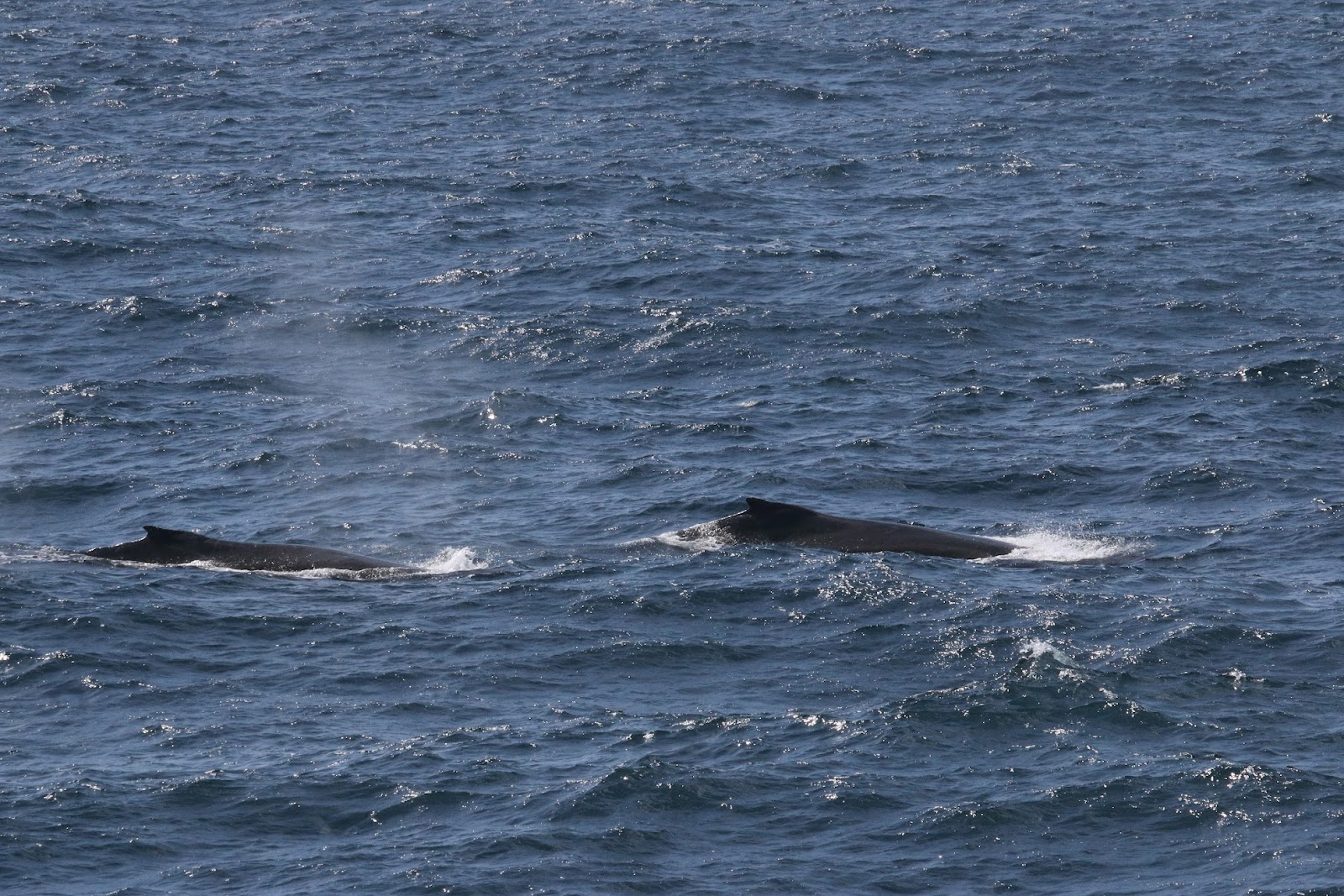
Observing whale behavior, such as for these humpbacks, provides valuable information on how they are using a given area.
One of the best experiences of the cruise for me was when we conducted a targeted net tow in an area of foraging humpbacks on the Heceta Head Line off the central Oregon coast. The combination of the krill signature I was seeing on the acoustics display, and the radio reports from Dawn and Clara of foraging dives, convinced me that this was an opportunity for a net tow, if possible, to see exactly what zooplankton was in the water near the whales. Our chief scientist, Jennifer Fisher, and the ship’s officers worked together to quickly turn the ship around and get a net in the water, in an effort to catch krill from the aggregation I had seen.
This unique opportunity gave me a chance to test my own interpretation of the acoustics data, and compare what we captured in the net with what I expected from the backscatter signal. It also prompted me to think more about the synchrony and differences between what is captured by net tows and echosounder data, two primary ways for looking at whale prey.
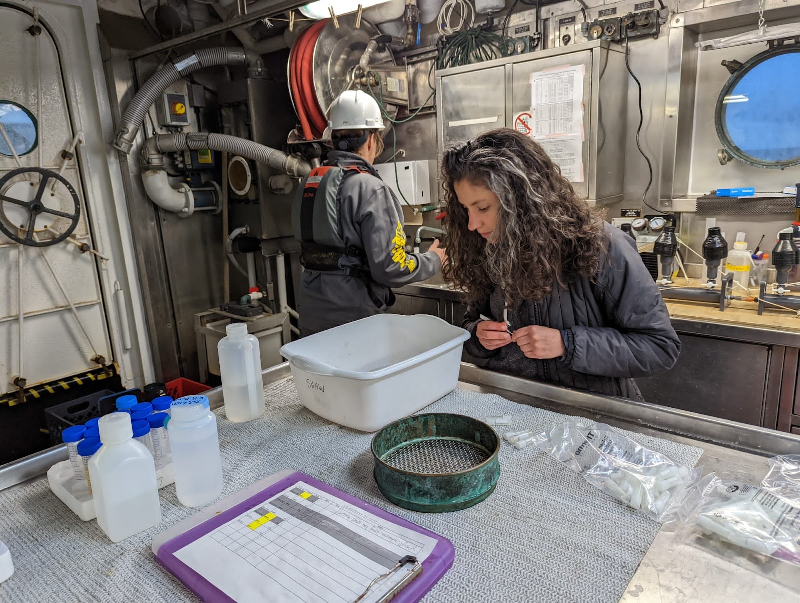
Collecting tiny yet precious krill samples associated with foraging humpbacks!
Throughout the entire cruise, the opportunity to build my intuition and notice ecological patterns was invaluable. Ecosystem modeling gives us the opportunity to untangle incredible complexity and put dynamic relationships in mathematical terms, but being out on the ocean provides the chance to develop a feel for these relationships. I’m so glad to bring this new perspective to my next round of models, and excited to continue trying to tease apart fine-scale dynamics between whales and krill.
Did you enjoy this blog? Want to learn more about marine life, research, and conservation? Subscribe to our blog and get a weekly message when we post a new blog. Just add your nameand email into the subscribe box below.
1PhD student, Oregon State University College of Earth, Ocean, and Atmospheric Sciences and Department of Fisheries, Wildlife, and Conservation Sciences, Geospatial Ecology of Marine Megafauna Lab
What do peanut butter m&ms, killer whales, affogatos, tired eyes, and puffins all have in common? They were all major features of the recent Northern California Current (NCC) ecosystem survey cruise.
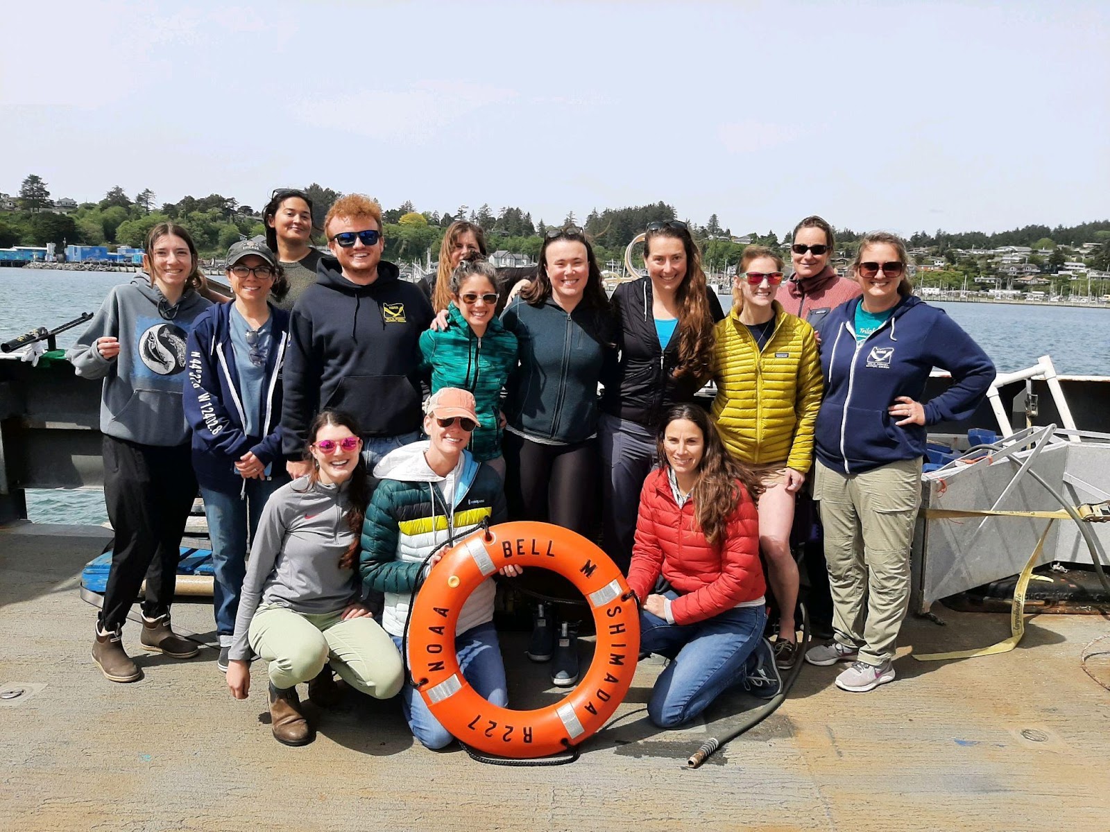
The science party of the May 2022 Northern California Current ecosystem cruise.
We spent May 6–17 aboard the NOAA vessel Bell M. Shimada in northern California, Oregon, and Washington waters. This fabulously interdisciplinary cruise studies multiple aspects of the NCC ecosystem three times per year, and the GEMM lab has put marine mammal observers aboard since 2018.
This cruise was a bit different than usual for the GEMM lab: we had eyes on both the whales and their prey. While Dawn Barlow and Clara Bird observed from sunrise to sunset to sight and identify whales, Rachel Kaplan collected krill data via an echosounder and samples from net tows in order to learn about the preyscape the whales were experiencing.
From left, Rachel, Dawn, and Clara after enjoying some beautiful sunset sightings.
We sailed out of Richmond, California and went north, sampling as far north as La Push, Washington and up to 200 miles offshore. Despite several days of challenging conditions due to wind, rain, fog, and swell, the team conducted a successful marine mammal survey. When poor weather prevented work, we turned to our favorite hobbies of coding and snacking.
Rachel attends “Clara’s Beanbag Coding Academy”.
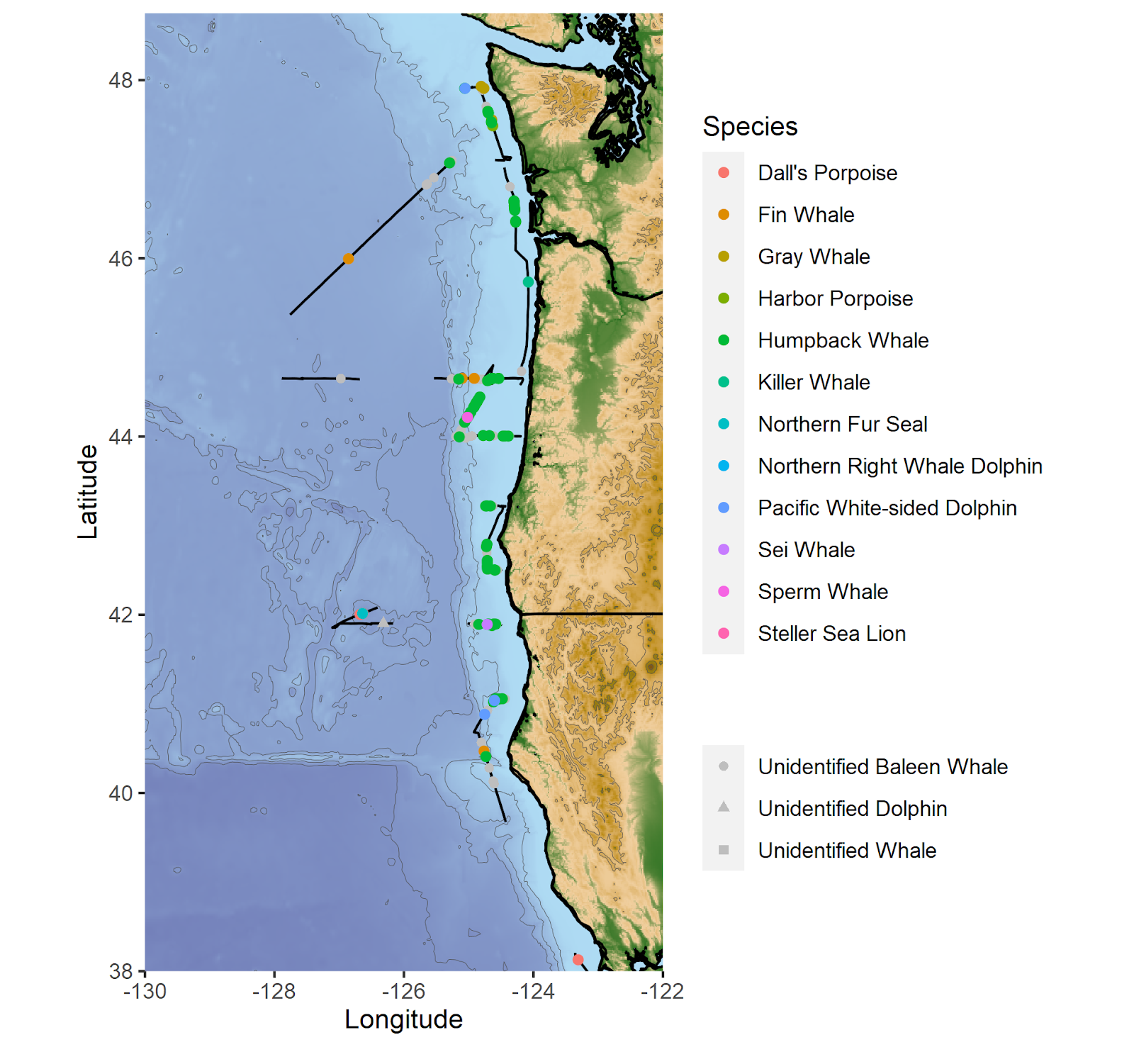
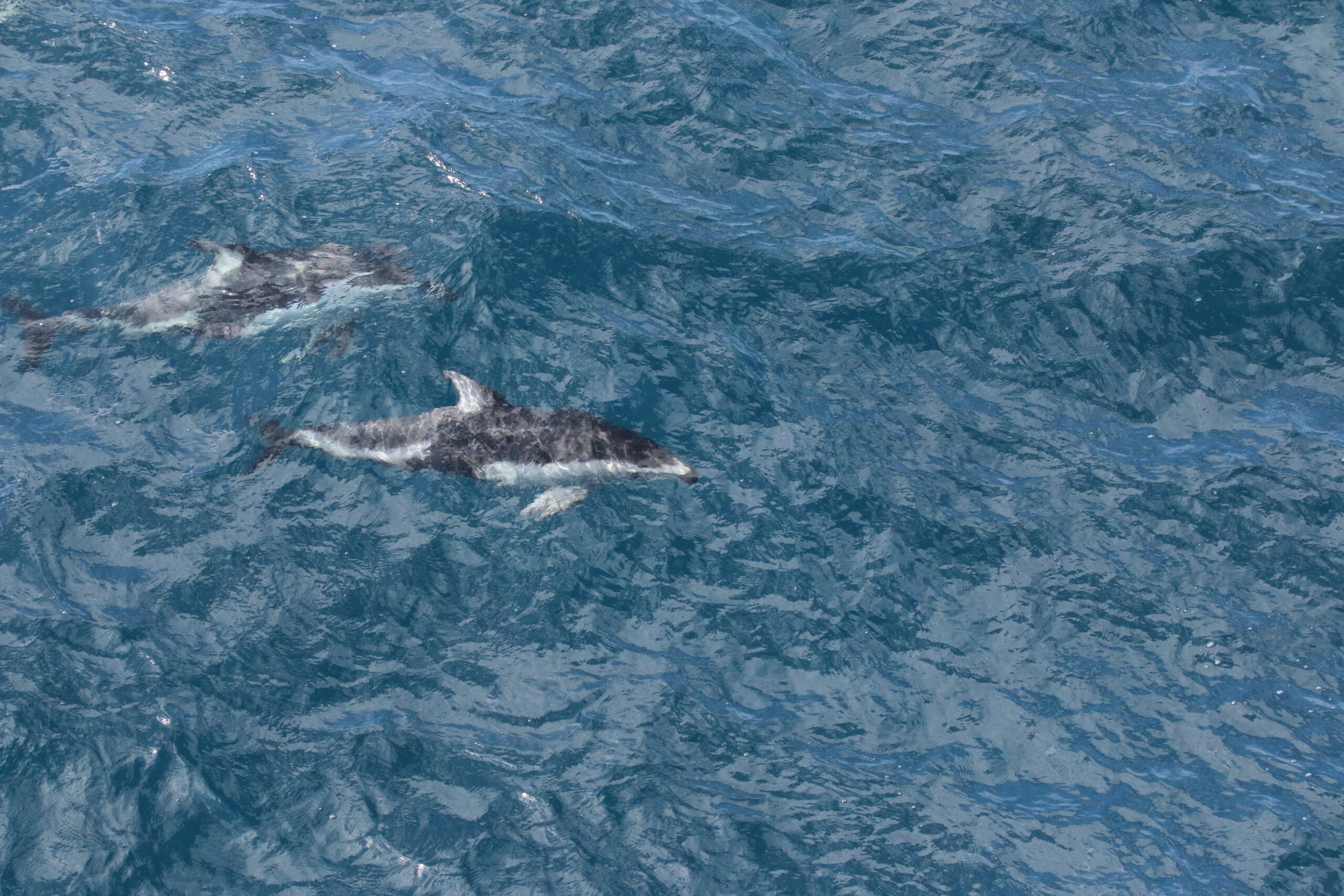
Cruise highlights included several fin whales, sperm whales, killer whales, foraging gray whales, fluke slapping and breaching humpbacks, and a visit by 60 pacific white-sided dolphins. While being stopped at an oceanographic sampling station typically means that we take a break from observing, having more time to watch the whales around us turned out to be quite fortunate on this cruise. We were able to identify two unidentified whales as sei whales after watching them swim near us while paused on station.
Marine mammal observation segments (black lines) and the sighting locations of marine mammal species observed during the cruise.
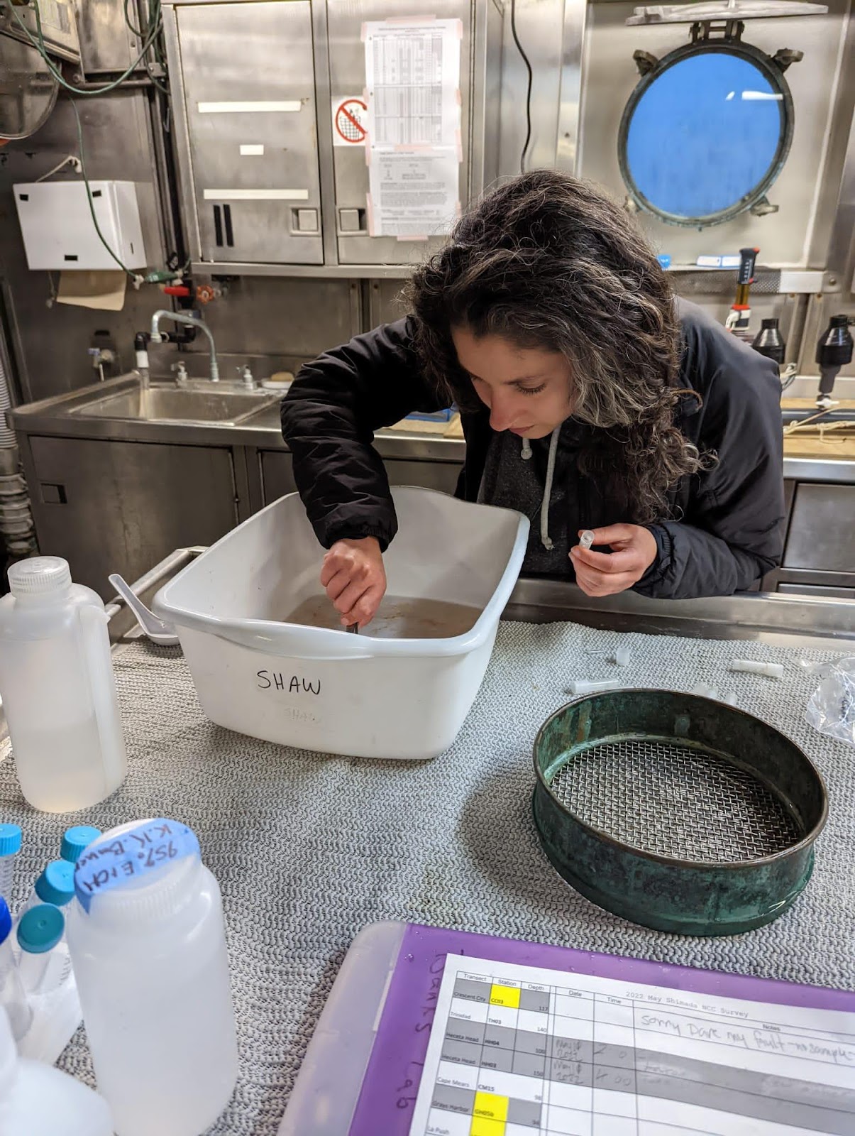
On one of our first survey days we also observed humpbacks surface lunge feeding close to the ship, which provided a valuable opportunity for our team to think about how to best collect concurrent prey and whale data. The opportunity to hone in on this predator-prey relationship presented itself in a new way when Dawn and Clara observed many apparently foraging humpbacks on the edge of Heceta Bank. At the same time, Rachel started observing concurrent prey aggregations on the echosounder. After a quick conversation with the chief scientist and the officers on the bridge, the ship turned around so that we could conduct a net tow in order to get a closer look at what exactly the whales were eating.
Success! Rachel collects krill samples collected in an area of foraging humpback whales.
This cruise captured an interesting moment in time: southerly winds were surprisingly common for this time of year, and the composition of the phytoplankton and zooplankton communities indicated that the seasonal process of upwelling had not yet been initiated. Upwelling brings deep, cold, nutrient-rich waters to the surface, generating a jolt of productivity that brings the ecosystem from winter into spring. It was fascinating to talk to all the other researchers on the ship about what they were seeing, and learn about the ways in which it was different from what they expected to see in May.
Experiencing these different conditions in the Northern California Current has given us a new perspective on an ecosystem that we’ve been observing and studying for years. We’re looking forward to digging into the data and seeing how it can help us understand this ecosystem more deeply, especially during a period of continued climate change.
The total number of each marine mammal species observed during the cruise.
Did you enjoy this blog? Want to learn more about marine life, research, and conservation? Subscribe to our blog and get a weekly message when we post a new blog. Just add your nameand email into the subscribe box below.
Pursuing a graduate degree as a member of the Marine Mammal Institute (MMI) comes with many advantages. Developing associations with curious, industrious researchers and working with advanced technological methods are certainly two of them. Particularly, as a member of the HALO project, I have the pleasure of working alongside not only the GEMM’s, but also acoustician Dr. Holger Klinck and his bioacoustics team at the K. Lisa Yang Center for Conservation Bioacoustics at the Cornell Lab (CCB) who have made significant contributions to advance the field for marine mammal research.
When the HALO project kicked off in October, 2021, Holger and graduate student, Marissa Garcia, arrived for our initial voyage off the Oregon coast with three specialized acoustic recording devices, called Rockhoppers. We deployed each Rockhopper at their designated locations, where they will remain and be replaced every six months, to collect continuous passive acoustic data of cetacean vocalizations. These data are significant because they gather information on all vocalizing whales and dolphins within a detectable range of the Rockhoppers, supporting not only my thesis work concerning fin whale distribution in the Northern California Current (NCC) but has the potential to inform multiple other research projects as well.
Figure 1. Craig Hayslip, Holger Klinck, and Marissa Garcia prepare a Rockhopper for deployment during the first HALO cruise off the Oregon coast.
Passive acoustic monitoring (PAM) is a non-invasive underwater method of recording acoustic output of cetaceans (Zimmer, 2011), and the Rockhopper is specialized for this task. The Rockhopper relatively small (each weighing ~90lbs.) and can be easily deployed with a minimal team from almost any vessel (Fig 1). The mooring is a simple system that anchors the Rockhopper to the sea floor after it sinks through the water column, tolerating depths up to 3,500 m (Klinck et al., 2020). The device can stay on the ocean floor for up to seven months continuously collecting high-frequency data (up to 197 kHz, 24 bits; Klinck et al., 2020). To recover the Rockhopper, the mooring system (Fig 2) includes an acoustic release; when the correct acoustic signal is transmitted by scientists from the vessel and received down at the seafloor, the Rockhopper is released. It’s positive buoyancy allows it to float to the surface where it is recovered. By developing the Rockhopper with these capabilities, the bioacoustics team at Cornell University have taken several steps to enhance cetacean research.
Figure 2. Rockhopper mooring system (Klinck et al., 2020).
According to one of it’s designers, David Winiarski, the Rockhopper development team, consisting of himself, Holger Klinck, Raymond Mack, Christopher Tessaglia-Hymes, Dmitri Ponirakis, Peter Dugan, Christopher Jones, and Haru Matsumoto, initiated it’s construction in 2015. Winiarski states that Jones developed the Rockhopper’s initial PAM electronics at Embedded Ocean Systems (EOS), Boston, MA and then the rest of the team developed the remainder of the device in 2017. The Rockhopper contains the electronic system and a 10.8 V Lithium battery pack in an oil-filled Vitrovex 43 cm glass sphere that is encased in hard polyethelene. Two 64 GB memory cards store the collected acoustic data. About every hour the internal processing unit moves the data to two 4 Terabyte solid-state drives in a process that ensures the data is not lost (Klinck et al., 2020). Winiarski attests that it was quite a hectic process to get six complete Rockhoppers ready for their initial deployment, however the team succeeded and in May 2018 they were deployed in the Gulf of Mexico. The Rockhoppers were recovered in 2019 after six months, returning an amazing 21,522 hours of continuous acoustic data (Klinck et al., 2020).
Learning this information about the acoustic devices that will be responsible for collecting my Master’s thesis data is encouraging. I am eager to see the fin whale energy captured within the Rockhopper records. The HALO team, along with myself, Holger, and Marissa, will head back out off the Oregon coast to retrieve our three HALO-designated Rockhoppers in early June (next month). We will then spend the summer at Cornell reading through our first six months of data.
So, why call this acoustic device, the “Rockhopper”? Winiarski explained that since the CCB is a subsect of the Cornell Lab of Ornithology their projects tend to be named after birds. The Rockhopper team thought that this device should respectively be named after a cool marine megafauna. Hence the rockhopper penguin was chosen. I do agree that such an outstanding device is well suited in relation with an equally remarkable marine species.
Left: Rockhopper penguins on a New Zealand hillside. https://nzbirdsonline.org.nz/species/eastern-rockhopper-penguin Upper right: Chris Tessaglia-Hymes and David Winiarski with a Rockhopper acoustic device. Lower right: The first six complete Rockhopper acoustic devices developed at the Cornell Center of Bioacoustics in 2017.
Did you enjoy this blog? Want to learn more about marine life, research, and conservation? Subscribe to our blog and get weekly updates and more! Just add your name into the subscribe box on the left panel.
References
Klinck, H., Winiarski, D., Mack, R., Tessaglia-Hymes, C., Ponirakis, D., Dugan, P., Jones, C., Matsumoto, H. 2020. The Rockhopper: a compact and extensible marine autonomous passive acoustic recording system,” Global Oceans 2020: Singapore – U.S. Gulf Coast: 1-7. https://ieeexplore.ieee.org/document/9388970.
Zimmer, W. 2011. Passive acoustic monitoring of cetaceans. Cambridge University Press, Cambridge, UK.
In September 2020, I was hired as a postdoc in the GEMM Lab and was tasked to conduct the analyses necessary for the OPAL project. This research project has the ambitious, yet essential, goal to fill a knowledge gap hindering whale conservation efforts locally: where and when do whales occur off the Oregon coast? Understanding and predicting whale distribution based on changing environmental conditions is a key strategy to assess and reduce spatial conflicts with human activities, specifically the risk of entanglement in fixed fishing gear.
Starting a new project is always a little daunting. Learning about a new region and new species, in an alien research and conservation context, is a challenge. As I have specialized in data science over the last couple of years, I have been confronted many times with the prospect of working with massive datasets collected by others, from which I was asked to tease apart the biases and the ecological patterns. In fact, I have come to love that part of my job: diving down the data rabbit hole and making my way through it by collaborating with others. Craig Hayslip, faculty research assistant in MMI, was the observer who conducted the majority of the 102 helicopter surveys that were used for this study. During the analysis stage, his help was crucial to understand the data that had been collected and get a better grasp of the field work biases that I would later have to account for in my models. Similarly, it took hours of zoom discussions with Dawn Barlow, the GEMM lab’s latest Dr, to be able to clean and process the 75 days of survey effort conducted at sea, aboard the R/V Shimada and Oceanus.
Once the data is “clean”, then comes the time for modeling. Running hundreds of models, with different statistical approaches, different environmental predictors, different parameters etc. etc. That is when you realize what a blessing it is to work with a supervisor like Leigh Torres, head of the GEMM Lab. As an early career researcher, I really appreciate working with people who help me take a step back and see the bigger picture within which the whole data wrangling work is included. It is so important to have someone help you stay focused on your goals and the ecological questions you are trying to answer, as these may easily get pushed back to the background during the data analysis process.
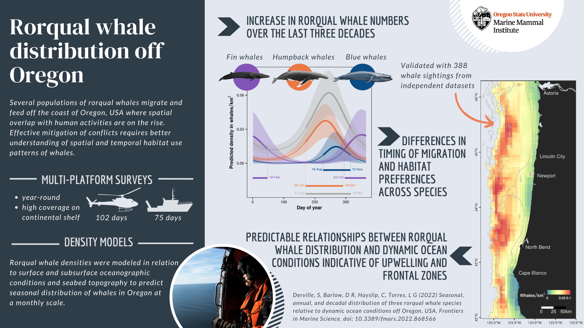
And here we are today, with the first scientific publication from the OPAL project published, a little more than three years after Leigh and Craig started collecting data onboard the United States Coast Guard helicopters off the coast of Oregon in February 2019. Entitled “Seasonal, annual, and decadal distribution of three rorqual whale species relative to dynamic ocean conditions off Oregon, USA”, our study published in Frontiers in Marine Science presents modern and fine-scale predictions of rorqual whale distribution off Oregon, as well as a description of their phenology and a comparison to whale numbers observed across three decades in the region (Figure 1). This research focuses on three rorqual species sharing some ecological and biological traits, as well as similar conservation status: humpback whales (Megaptera novaeangliae), blue whales (Balaenoptera musculus musculus), and fin whales (Balaenoptera physallus); all of which migrate and feed over the US West coast (see a previous blog to learn more about these species here).
Figure 1: Graphical abstract of our latest paper published in Frontiers in Marine Science.
We demonstrate (1) an increase in rorqual numbers over the last three decades in Oregon waters, (2) differences in timing of migration and habitat preferences between humpback, blue, and fin whales, and (3) predictable relationships of rorqual whale distribution based on dynamic ocean conditions indicative of upwellings and frontal zones. Indeed, these ocean conditions are likely to provide suitable biological conditions triggering increased prey abundance. Three seasonal models covering the months of December-March (winter model), April-July (spring) and August-November (summer-fall) were generated to predict rorqual whale densities over the Oregon continental shelf (in waters up to 1,500 m deep). As a result, maps of whale densities can be produced on a weekly basis at a resolution of 5 km, which is a scale that will facilitate targeted management of human activities in Oregon. In addition, species-specific models were also produced over the period of high occurrence in the region; that is humpback and blue whales between April and November, and fin whales between August and March.
As we outline in our concluding remarks, this work is not to be considered an end-point, but rather a stepping stone to improve ecological knowledge and produce operational outputs that can be used effectively by managers and stakeholders to prevent spatial conflict between whales and human activities. As of today, the models of fin and blue whale densities are limited by the small number of observations of these two species over the Oregon continental shelf. Yet, we hope that continued data collection via fruitful research partnerships will allow us to improve the robustness of these species-specific predictions in the future. On the other hand, the rorqual models are considered sufficiently robust to continue into the next phase of the OPAL project that aims to assess overlap between whale distribution and Dungeness crab fishing gear to estimate entanglement risk.
The curse (or perhaps the beauty?) of species distribution modeling is that it never ends. There are always new data to be added, new statistical approaches to be tested, and new predictions to be made. The OPAL models are no exception to this rule. They are meant to be improved in future years, thanks to continued helicopter and ship-based survey efforts, and to the addition of new environmental variables meant to better predict whale habitat selection. For instance, Rachel Kaplan’s PhD research specifically aims at understanding the distribution of whales in relation to krill. Her results will feed into the more general efforts to model and predict whale distribution to inform management in Oregon.
This first publication therefore paves the way for more exciting and impactful research!
Did you enjoy this blog? Want to learn more about marine life, research, and conservation? Subscribe to our blog and get a weekly message when we post a new blog. Just add your name and email into the subscribe box below.
Reference
Derville, S., Barlow, D. R., Hayslip, C. E., and Torres, L. G. (2022). Seasonal, Annual, and Decadal Distribution of Three Rorqual Whale Species Relative to Dynamic Ocean Conditions Off Oregon, USA. Front. Mar. Sci. 9, 1–19. doi:10.3389/fmars.2022.868566.
Acknowledgments
We gratefully acknowledge the immense contribution of the United State Coast Guard sectors North Bend and Columbia River who facilitated and piloted our helicopter surveys. We would like to also thank NOAA Northwest Fisheries Science Center for the ship time aboard the R/V Bell M. Shimada. We thank the R/V Bell M. Shimada (chief scientists J. Fisher and S. Zeman) and R/V Oceanus crews, as well as the marine mammal observers F. Sullivan, C. Bird and R. Kaplan. We give special recognition and thanks to the late Alexa Kownacki who contributed so much in the field and to our lives. We also thank T. Buell and K. Corbett (ODFW) for their partnership over the OPAL project. We thank G. Green and J. Brueggeman (Minerals Management Service), J. Adams (US Geological Survey), J. Jahncke (Point blue Conservation), S. Benson (NOAA-South West Fisheries Science Center), and L. Ballance (Oregon State University) for sharing validation data. We thank J. Calambokidis (Cascadia Research Collective) for sharing validation data and for logistical support of the project. We thank A. Virgili for sharing advice and custom codes to produce detection functions.
Dr. KC Bierlich, Postdoctoral Scholar, OSU Department of Fisheries, Wildlife, & Conservation Sciences, Geospatial Ecology of Marine Megafauna (GEMM) Lab
In a previous blog, I discussed the importance of incorporating measurement uncertainty in drone-based photogrammetry, as drones with different sensors, focal length lenses, and altimeters will have varying levels of measurement accuracy. In my last blog, I discussed how to incorporate photogrammetric uncertainty when combining multiple measurements to estimate body condition of baleen whales. In this blog, I will highlight our recent publication in Frontiers in Marine Science (https://doi.org/10.3389/fmars.2022.867258) led by GEMM Lab’s Dr. Leigh Torres, Clara Bird, and myself that used these methods in a collaborative study using imagery from four different drones to compare gray whale body condition on their breeding and feeding grounds (Torres et al., 2022).
Most Eastern North Pacific (ENP) gray whales migrate to their summer foraging grounds in Alaska and the Arctic, where they target benthic amphipods as prey. A subgroup of gray whales (~230 individuals) called the Pacific Coast Feeding Group (PCFG), instead truncates their migration and forages along the coastal habitats between Northern California and British Columbia, Canada (Fig. 1). Evidence from a recent study lead by GEMM Lab’s Lisa Hildebrand (see this blog) found that the caloric content of prey in the PCFG range is of equal or higher value than the main amphipod prey in the Arctic/sub-Arctic regions (Hildebrand et al., 2021). This implies that greater prey density and/or lower energetic costs of foraging in the Arctic/sub-Arctic may explain the greater number of whales foraging in that region compared to the PCFG range. Both groups of gray whales spend the winter months on their breeding and calving grounds in Baja California, Mexico.
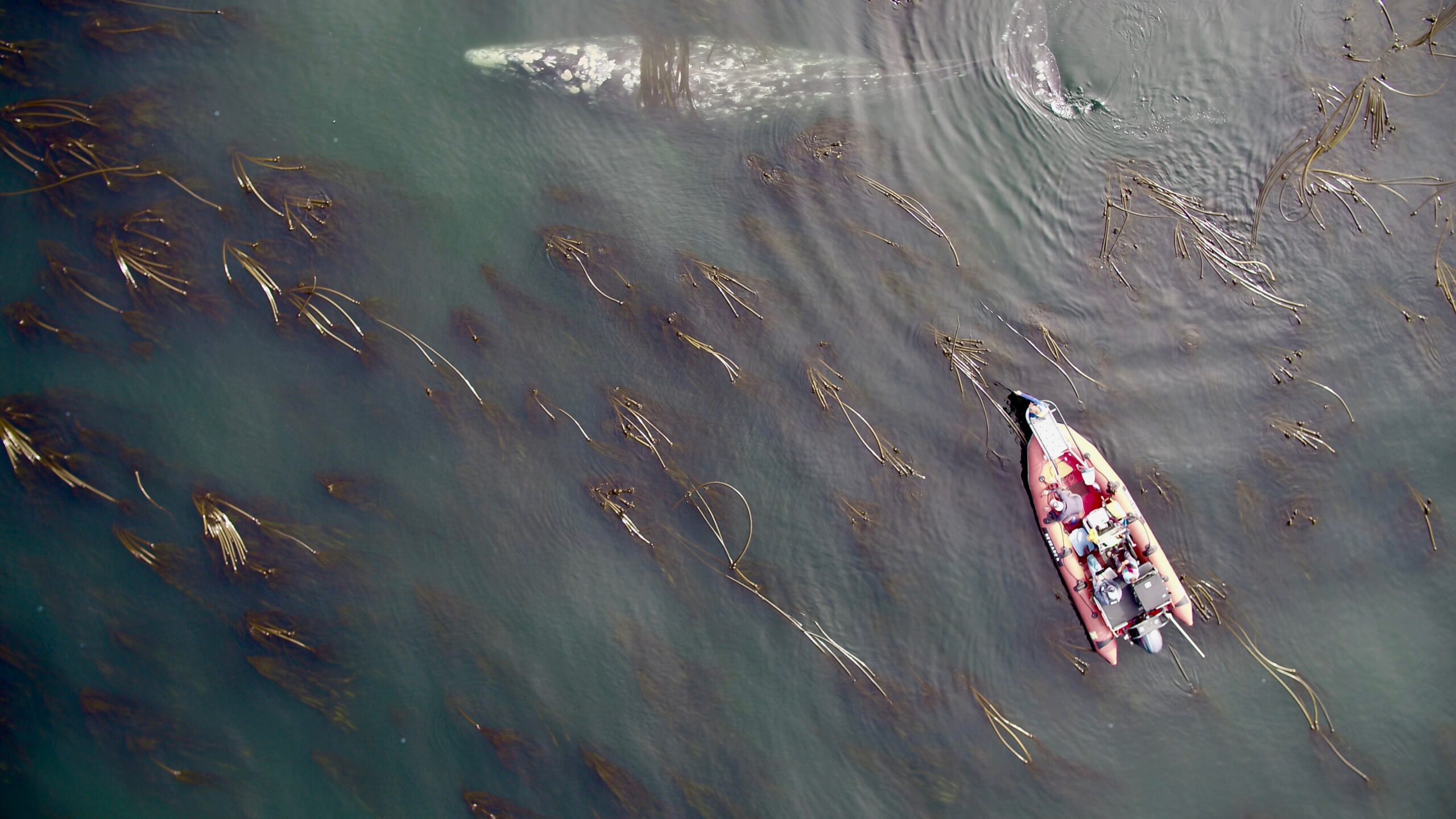
Figure 1. The GEMM Lab field team following a Pacific Coast Feeding Group (PCFG) gray whale swimming in a kelp bed along the Oregon Coast during the summer foraging season.
In January 2019 an Unusual Mortality Event (UME) was declared for gray whales due to the elevated numbers of stranded gray whales between Mexico and the Arctic regions of Alaska. Most of the stranded whales were emaciated, indicating that reduced nutrition and starvation may have been the causal factor of death. It is estimated that the population dropped from ~27,000 individuals in 2016 to ~21,000 in 2020 (Stewart & Weller, 2021).
During this UME period, between 2017-2019, the GEMM Lab was using drones to monitor the body condition of PCFG gray whales on their Oregon coastal feeding grounds (Fig. 1), while Christiansen and colleagues (2020) was using drones to monitor gray whales on their breeding grounds in San Ignacio Lagoon (SIL) in Baja California, Mexico. We teamed up with Christiansen and colleagues to compare the body condition of gray whales in these two different areas leading up to the UME. Comparing the body condition between these two populations could help inform which population was most effected by the UME.
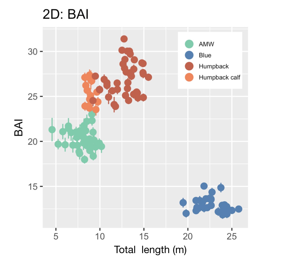
The combined datasets consisted of four different drones used, thus different levels of photogrammetric uncertainty to consider. The GEMM Lab collected data using a DJI Phantom 3 Pro, DJI Phantom 4, and DJI Phantom 4 Pro, while Christiansen et al., (2020) used a DJI Inspire 1 Pro. By using the methodological approach described in my previous blog (here, also see Bierlich et al., 2021a for more details), we quantified photogrammetric uncertainty specific to each drone, allowing cross-comparison between these datasets. We also used Body Area Index (BAI), which is a standardized relative measure of body condition developed by the GEMM Lab (Burnett et al., 2018) that has low uncertainty with high precision, making it easier to detect smaller changes between individuals (see blog here, Bierlich et al., 2021b).
While both PCFG and ENP gray whales visit San Ignacio Lagoon in the winter, we assume that the photogrammetry data collected in the lagoon is mostly of ENP whales based on their considerably higher population abundance. We also assume that gray whales incur low energetic cost during migration, as gray whale oxygen consumption rates and derived metabolic rates are much lower during migration than on foraging grounds (Sumich, 1983).
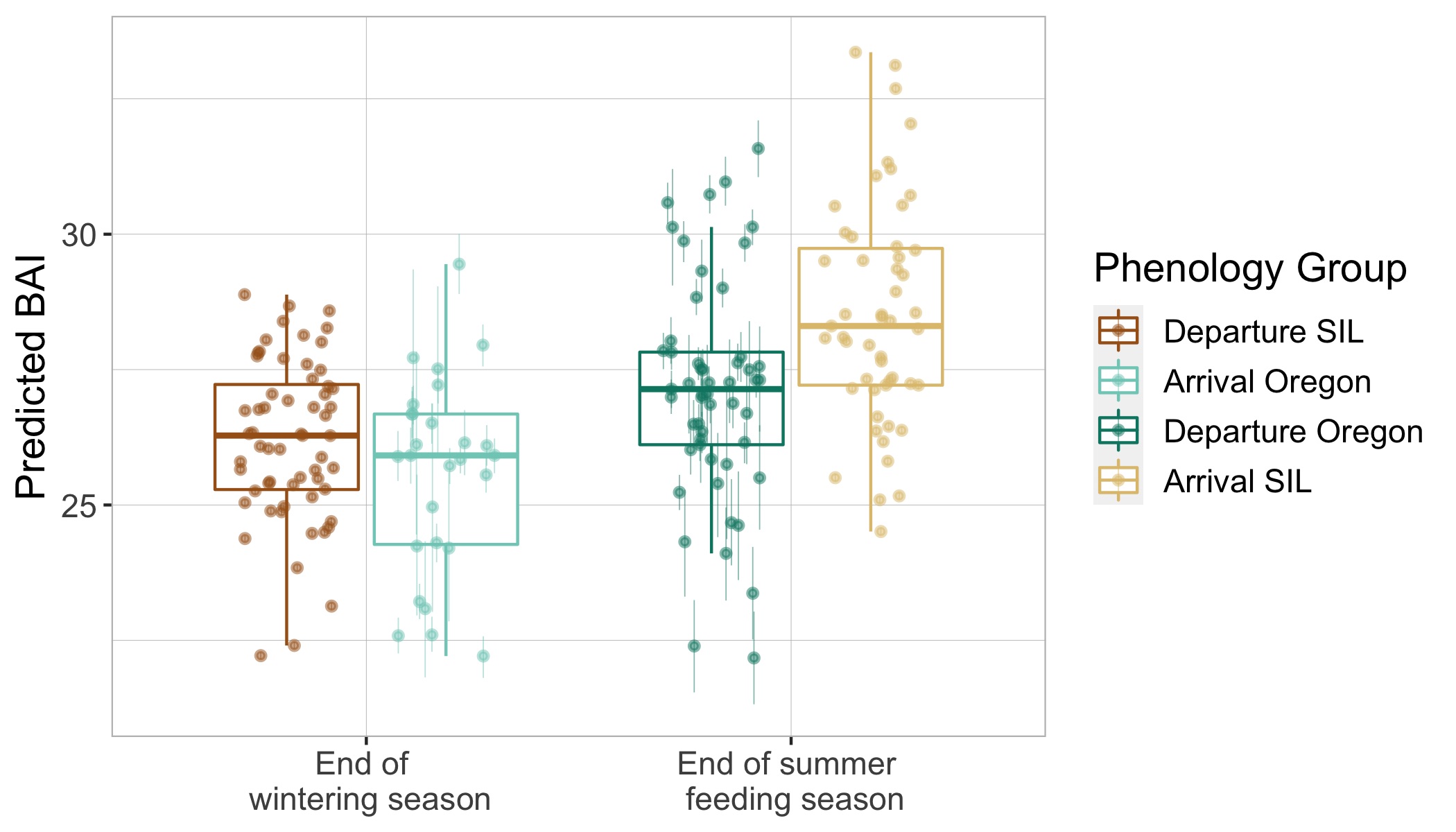
Interestingly, we found that gray whale body condition on their wintering grounds in San Ignacio Lagoon deteriorated across the study years leading up to the UME (2017-2019), while the body condition of PCFG whales on their foraging grounds in Oregon concurrently increased. These contrasting trajectories in body condition between ENP and PCFG whales implies that dynamic oceanographic processes may be contributing to temporal variability of prey available in the Arctic/sub-Arctic and PCFG range. In other words, environmental conditions that control prey availability for gray whales are different in the two areas. For the ENP population, this declining nutritive gain may be associated with environmental changes in the Arctic/sub-Arctic region that impacted the predictability and availability of prey. For the PCFG population, the increase in body condition across years may reflect recovery of the NE Pacific Ocean from the marine heatwave event in 2014-2016 (referred to as “The Blob”) that resulted with a period of low prey availability. These findings also indicate that the ENP population was primarily impacted in the die-off from the UME.
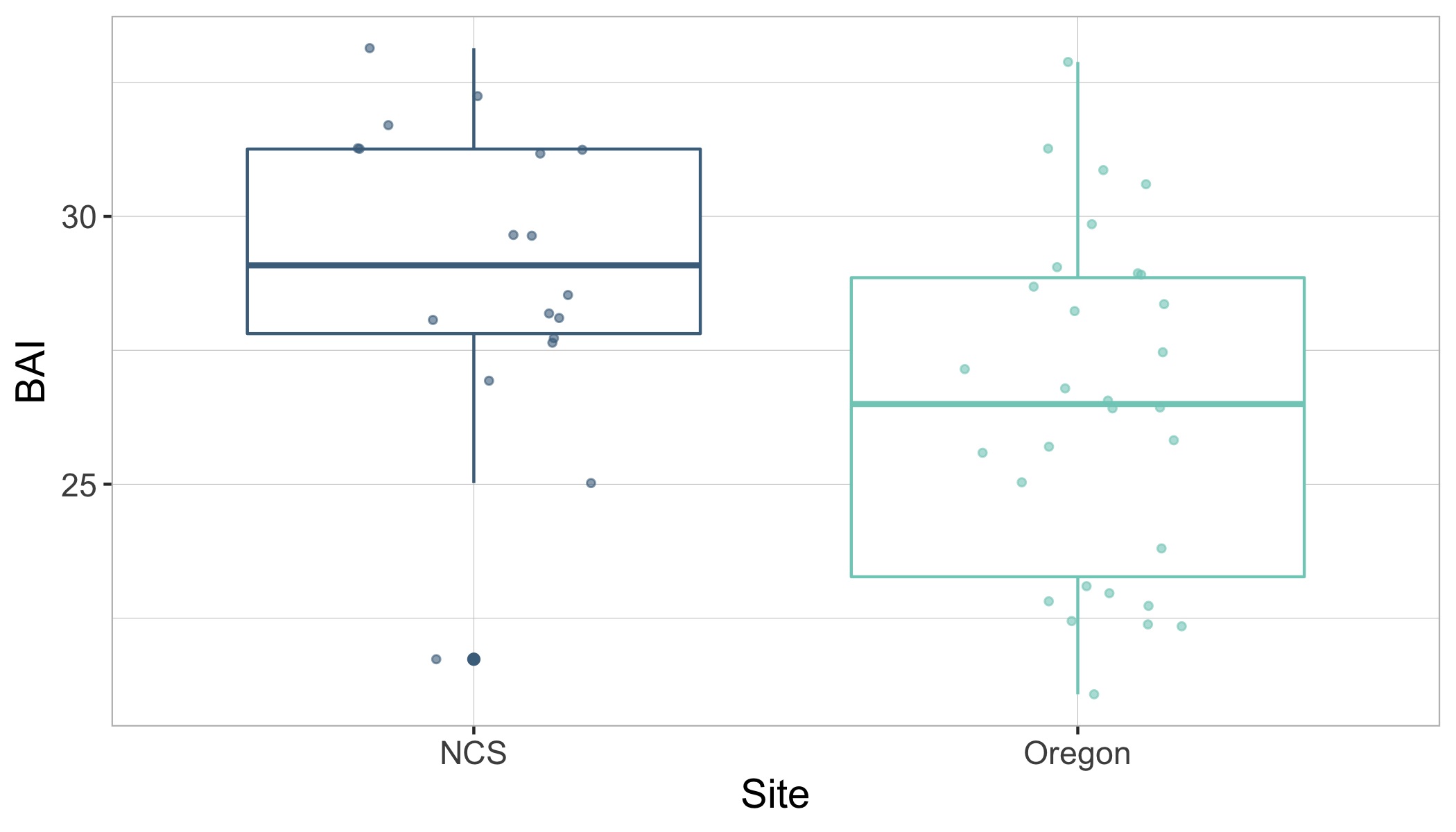
Surprisingly, the body condition of PCFG gray whales in Oregon was regularly and significantly lower than whales in San Ignacio Lagoon (Fig. 2). To further investigate this potential intrinsic difference in body condition between PCFG and ENP whales, we compared opportunistic photographs of gray whales feeding in the Northeastern Chukchi Sea (NCS) in the Arctic collected from airplane surveys. We found that the body condition of PCFG gray whales was significantly lower than whales in the NCS, further supporting our finding that PCFG whales overall have lower body condition than ENP whales that feed in the Arctic (Fig. 3).
Figure 2. Boxplots showing the distribution of Body Area Index (BAI) values for gray whales imaged by drones in San Ignacio Lagoon (SIL), Mexico and Oregon, USA. The data is grouped by phenology group: End of summer feeding season (departure Oregon vs. arrival SIL) and End of wintering season (arrival Oregon vs. departure SIL). The group median (horizontal line), interquartile range (IQR, box), maximum and minimum 1.5*IQR (vertical lines), and outliers (dots) are depicted in the boxplots. The overlaid points represent the mean of the posterior predictive distribution for BAI of an individual and the bars represents the uncertainty (upper and lower bounds of the 95% HPD interval). Note how PCFG whales at then end of the feeding season (dark green) typically have lower body condition (as BAI) compared to ENP whales at the end of the feeding season when they arrive to SIL after migration (light brown).Figure 3. Boxplots showing the distribution of Body Area Index (BAI) values of gray whales from opportunistic images collected from a plane in Northeaster Chukchi Sea (NCS) and from drones collected by the GEMM Lab in Oregon. The boxplots display the group median (horizontal line), interquartile range (IQR box), maximum and minimum 1.5*IQR (vertical lines), and outlies (dots). The overlaid points are the BAI values from each image. Note the significantly lower BAI of PCFG whales on Oregon feeding grounds compared to whales feeding in the Arctic region of the NCS.
This difference in body condition between PCFG and ENP gray whales raises some really interesting and prudent questions. Does the lower body condition of PCFG whales make them less resilient to changes in prey availability compared to ENP whales, and thus more vulnerable to climate change? If so, could this influence the reproductive capacity of PCFG whales? Or, are whales that recruit into the PCFG adapted to a smaller morphology, perhaps due to their specialized foraging tactics, which may be genetically inherited and enables them to survive with reduced energy stores?
These questions are on our minds here at the GEMM Lab as we prepare for our seventh consecutive field season using drones to collect data on PCFG gray whale body condition. As discussed in a previous blog by Dr. Alejandro Fernandez Ajo, we are combining our sightings history of individual whales, fecal hormone analyses, and photogrammetry-based body condition to better understand gray whales’ reproductive biology and help determine what the consequences are for these PCFG whales with lower body condition.
Did you enjoy this blog? Want to learn more about marine life, research, and conservation? Subscribe to our blog and get a weekly message when we post a new blog. Just add your name and email into the subscribe box below.
References
Bierlich, K. C., Hewitt, J., Bird, C. N., Schick, R. S., Friedlaender, A., Torres, L. G., … & Johnston, D. W. (2021). Comparing Uncertainty Associated With 1-, 2-, and 3D Aerial Photogrammetry-Based Body Condition Measurements of Baleen Whales. Frontiers in Marine Science, 1729.
Bierlich, K. C., Schick, R. S., Hewitt, J., Dale, J., Goldbogen, J. A., Friedlaender, A.S., et al. (2021b). Bayesian Approach for Predicting Photogrammetric Uncertainty in Morphometric Measurements Derived From Drones. Mar. Ecol. Prog. Ser. 673, 193–210. doi: 10.3354/meps13814
Burnett, J. D., Lemos, L., Barlow, D., Wing, M. G., Chandler, T., & Torres, L. G. (2018). Estimating morphometric attributes of baleen whales with photogrammetry from small UASs: A case study with blue and gray whales. Marine Mammal Science, 35(1), 108–139.
Christiansen, F., Rodrı́guez-González, F., Martı́nez-Aguilar, S., Urbán, J., Swartz, S., Warick, H., et al. (2021). Poor Body Condition Associated With an Unusual Mortality Event in Gray Whales. Mar. Ecol. Prog. Ser. 658, 237–252. doi:10.3354/meps13585
Hildebrand, L., Bernard, K. S., and Torres, L. G. (2021). Do Gray Whales Count Calories? Comparing Energetic Values of Gray Whale Prey Across Two Different Feeding Grounds in the Eastern North Pacific. Front. Mar. Sci. 8. doi: 10.3389/fmars.2021.683634
Stewart, J. D., and Weller, D. (2021). Abundance of Eastern North Pacific Gray Whales 2019/2020 (San Diego, CA: NOAA/NMFS)
Sumich, J. L. (1983). Swimming Velocities, Breathing Patterns, and Estimated Costs of Locomotion in Migrating Gray Whales, Eschrichtius Robustus. Can. J. Zoology. 61, 647–652. doi: 10.1139/z83-086
Torres, L.G., Bird, C., Rodrigues-Gonzáles, F., Christiansen F., Bejder, L., Lemos, L., Urbán Ramírez, J., Swartz, S., Willoughby, A., Hewitt., J., Bierlich, K.C. (2022). Range-wide comparison of gray whale body condition reveals contrasting sub-population health characteristics and vulnerability to environmental change. Frontiers in Marine Science. 9:867258. https://doi.org/10.3389/fmars.2022.867258
Allison Dawn, GEMM Lab Master’s student, OSU Department of Fisheries, Wildlife and Conservation Sciences, Geospatial Ecology of Marine Megafauna Lab
As the first year of my Master’s is coming to an end, I am excited to have completed the first milestone of writing my research proposal. During the formation of my initial hypotheses, I have been thinking deeply about the potential drivers of zooplankton variability, and how these metrics relate to the Pacific Coast Feeding Group (PCFG) of gray whales foraging in Port Orford. One topic that continues to appear in the literature and throughout my coursework is that of the extreme marine heat wave (MHW) event (2013-2016) in the Pacific Ocean, otherwise known as the “warm blob”. In Dawn’s (now Dr. Barlow!) blog about this MHW, she discusses how whale habitat in California was compressed due to shifts in prey availability, and how this led to an increased number of whale entanglements (Santora et al., 2020). While sea surface temperature (SST) is only one of many factors that influence prey metrics, it is nevertheless an important factor to consider, especially as these heat waves are expected to increase in intensity and duration due to climate change (Joh and Di Lorenzo, 2017). As Lisa mentioned in her last blog, the “warm blob” exacerbated the loss of kelp and sea stars, which is now impacting multiple trophic levels in Port Orford. For my first thesis chapter, I plan to dive into how SST anomalies impact the mosaic of interactions at our study site in Port Orford, and ultimately try to better understand food availability for the PCFG whales.
Cavole et al., 2016 is one of the early comprehensive studies to discuss the impact of the blob on a variety of planktonic marine species. Their sea surface temperature anomaly figure (Figure 1) shows where the anomaly began in 2013 and how it migrated from the Northern Pacific to the Southern Pacific coast.
Figure 1. Plots showing the SST anomalies as the “warm blob” migrated from the Northern Pacific to the Southern Pacific from 2013 until 2016.
Among many other impacts, this MHW caused a reduction in phytoplankton, the major food source for zooplankton. The decline of this food source subsequently caused significant changes in zooplankton populations. Specifically, studies on copepod diversity and biomass show that in a typical California Current System (CCS) there is a seasonal oscillation between warm-water with subtropical species and cold-water with subarctic species. In the winter, the CCS is characterized by a high diversity of subtropical species, due to a southern water source. In the spring, northern cold water advection brings low-diversity, subarctic copepods. While the timing of these shifts is subject to change due to changes in the Pacific Decadal Oscillation (PDO), it remains that these subtropical copepod species are known to be smaller and less nutritious than subarctic copepod species regardless of arrival time (Kintisch, 2015; Leising et al., 2015). However, in 2015, this shift to cold water copepod species did not occur, but rather coastal sampling along the Oregon coast saw subtropical copepod species prevail. Specifically, there were 17 main subtropical copepod species that dominated the species composition while the nutrient-rich arctic species were rare. This occurrence of major copepod shifts alone points to the overall concern for the ecosystem imbalance, to the detriment of top predators like marine mammals and seabirds (the “losers”), and others gaining advantage (the “winners”) (Figure 2).
Figure 2. Figure showing the “losers” (right column) and “winners” (left column) of MHW impacts. Species are organized by trophic level, with top predators at the bottom. Taken from Cavole et al., 2016.
More recent studies found that in certain areas, impacts from the “warm blob” outlived the duration of the larger scale anomaly. In fact, large, positive SST anomalies have lingered on the Oregon shelf until at least September 2017 (Peterson et al., 2017). During this time period, anomalously high abundances of nearshore larval North Pacific krill (Euphausia pacifica) were collected off of the Newport Hydrographic Station (Morgan et al., 2019). Additionally, Brodeur et al. (2019) demonstrate that while indicator species in the nearshore have consistent annual variability, there were substantial differences between community composition between 2011-2014 (low diversity) and 2015-2016 (high diversity). This work also documented the shift from crustacean species (like krill and mysids) to more low-quality gelatinous taxa. As the authors acknowledge, this change in prey community assemblage could have major negative impacts on trophic interactions. This is especially true in the context of whales, as they are not known to rely on gelatinous taxa for energy.
Just like our summer sampling in Port Orford, these studies only provide a “snapshot” of plankton species abundance and composition during a particular time of year. However, even a snapshot can reveal significant changes in prey variability, which then may help us understand the drivers of PCFG habitat utilization. We are actively investigating whether there have been significant changes in the variability of several zooplankton metrics (abundance, distribution, size class, composition) relative to SST changes in Port Orford over the last 6 years (2016-2021).
We will also consider multiple other static and dynamic factors that could influence zooplankton patterns (e.g., upwelling strength, kelp health, tidal height, topography); however, given these documented strong relationships between the zooplankton community and SST across the North Pacific, we hypothesize similar impacts in our Port Orford study region. For example, in certain sampling years, net tows seemed to be comprised of smaller size classes of zooplankton than usual. We will consider how size class availability has changed and if this was driven by SST variability. Gray whales are drawn to this area for enhanced feeding opportunities, and understanding the drivers of zooplankton, especially high quality prey, is a key step to understanding whale use of the area.
Please stay tuned for more updates as we continue working towards the answer to these pressing questions!
Did you enjoy this blog? Want to learn more about marine life, research, and conservation? Subscribe to our blog and get a weekly message when we post a new blog. Just add your name and email into the subscribe box below.
References
Brodeur, R. D., Auth, T. D., & Phillips, A. J. (2019). Major shifts in pelagic micronekton and macrozooplankton community structure in an upwelling ecosystem related to an unprecedented marine heatwave. Frontiers in Marine Science, 6, 212.
Cavole, L. M., Demko, A. M., Diner, R. E., Giddings, A., Koester, I., Pagniello, C. M., … & Franks, P. J. (2016). Biological impacts of the 2013–2015 warm-water anomaly in the Northeast Pacific: winners, losers, and the future. Oceanography, 29(2), 273-285.
Joh, Y., & Di Lorenzo, E. (2017). Increasing coupling between NPGO and PDO leads to prolonged marine heatwaves in the Northeast Pacific. Geophysical Research Letters, 44(22), 11-663.
Kintisch, E. (2015). ‘The Blob’ invades Pacific, flummoxing climate experts.
Leising, A. W., Schroeder, I. D., Bograd, S. J., Abell, J., Durazo, R., Gaxiola-Castro, G., … & Warybok, P. (2015). State of the California Current 2014-15: Impacts of the Warm-Water” Blob”. California Cooperative Oceanic Fisheries Investigations Reports, 56.
Morgan, C. A., Beckman, B. R., Weitkamp, L. A., & Fresh, K. L. (2019). Recent ecosystem disturbance in the Northern California current. Fisheries, 44(10), 465-474.
NOAA Fisheries. 2015b. California Current Integrated Ecosystem Assessment (CCIEA) State of the California Current Report, 2015. NMFS Report 2. Santora, J. A., Mantua, N. J., Schroeder, I. D., Field, J. C., Hazen, E. L., Bograd, S. J., … & Forney, K. A. (2020). Habitat compression and ecosystem shifts as potential links between marine heatwave and record whale entanglements. Nature communications, 11(1), 1-12.
When I was younger, I aspired to be a marine mammal biologist. I thought it was purely about knowing as much about marine mammal species as possible. However, over time and with experience in this field, I have realized that in order to understand a species, you need to have a holistic understanding of its prey, habitat, and environment. When I first applied to be advised by Leigh in the GEMM Lab, I had no idea how much of my time I would spend looking at tiny zooplankton under a microscope, thinking about the different benefits of different habitat types, or reading about oceanographic processes. But these things have been incredibly vital to my research to date and as a result, I now refer to myself as a marine ecologist. This holistic understanding that I am gaining will only grow throughout my PhD as I am broadly looking at the habitat use, site fidelity, and population dynamics of the Pacific Coast Feeding Group (PCFG) of gray whales for my thesis research.
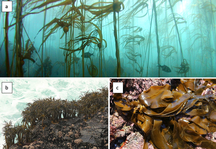
The PCFG display many foraging tactics and occupy several habitat types along the Oregon coast while they spend their summer feeding seasons here (Torres et al. 2018). Here, I will focus on one of these habitats: kelp. When you hear the word kelp, you probably conjure an image of long, thick stalks that reach from the ocean floor to the surface, with billowing fronds waving around (Figure 1a). However, this type is only one of three basic morphologies (Filbee-Dexter & Scheibling 2014) and it is called canopy kelp, which often forms extensive forests. The other two morphologies are stipitate and prostrate kelps. The former forms midwater stands (Figure 1b) while the latter forms low-lying kelp beds (Figure 1c). All three of these morphologies exist on the Oregon coast and create a mosaic of understory and canopy kelp patches that dot our coastline.
Figure 1. Examples of the three different kelp morphologies. a: bull kelp (Nereocystis luetkeana) is a type of canopy kelp and the dominant kelp on the Oregon coast (Source: Oregon Coast Aquarium); b: sea palm (Postelsia palmaeformis) is a type of stipitate kelp that forms mid-water stands (Source: Oregon Conservation Strategy); c: sea cabbage (Saccharina sessilis) is a type of prostrate kelp that is stipeless and forms low-lying kelp beds (Source: Central Coast Biodiversity).
One of the most magnificent things about kelp is that it is not just a species itself, but it provides critical habitat, refuge, and food resources to a myriad of other species due to its high rates of primary production (Dayton 1985). Kelp is often referred to as a foundation species due to all of these critical services it provides. In Oregon, many species of rockfish, which are important commercial and recreational fisheries, use kelp as habitat throughout their life cycle, including as nursery grounds. Lingcod, another widely fished species, forages amongst kelp. A large number of macroinvertebrates can be found in Oregon kelp forests, including anemones, limpets, snails, sea urchins, sea stars, and abalone, to name a fraction of them.
Kelps grow best in cold, nutrient-rich waters (Tegner et al. 1996) and their growth and distribution patterns are highly naturally variable on both temporal and spatial scales (Krumhansl et al. 2016). However, warm water, low nutrient or light conditions, intensive grazing by herbivores, and severe storm activity can lead to the erosion and defoliation of kelp beds (Krumhansl et al. 2016). While these events can occur naturally in cyclical patterns, the frequency of several of these events has increased in recent years, as a result of climate change and anthropogenic impacts. For example, Dawn’s blog discussed increasing marine heatwaves that represent an influx of warm water for a prolonged period of time. In fact, kelps can be useful sentinels of change as they tend to be highly responsive to changes in environmental conditions (e.g., Rogers-Bennet & Catton 2019) and their nearshore, coastal location directly exposes them to human activities, such as pollution, harvesting, and fishing (Bennett et al. 2016).
Due to its foundational role, changes or impacts to kelp can reverberate throughout the ecosystem and negatively affect many other species. As mentioned previously, kelp is naturally highly variable, and like many other ecological processes, undergoes boom and bust cycles. For over four decades, dense, productive kelp forests have been shown to transition to sea urchin barrens, and back again, in natural cycles (Sala et al. 1998;Pinnegar et al. 2000;Steneck et al. 2002; Figure 2). These transitions are called phase shifts. In a healthy, balanced kelp forest, sea urchins typically passively feed on detrital plant matter, such as broken off pieces of kelp fronds that fall to the seafloor. A phase shift occurs when the grazing intensity of sea urchins increases, resulting in them actively feeding on kelp stalks and fronds to a point where the kelp in an area can become greatly reduced, creating an urchin barren. Sea urchin grazing intensity can change for a number of reasons, including reduction in sea urchin predators (e.g., sea otters, sunflower sea stars) or poor kelp recruitment events (e.g., due to warm water temperature). Regardless of the reason, the phases tend to transition back and forth over time. However, there is concern that sea urchin barrens may become an alternative stable state of the subtidal ecosystem from which kelp in an area cannot recover (Filbee-Dexter & Scheibling 2014).
Figure 2. Screenshots from GoPro videos from 2016 (left) and 2018 (right) at the same kayak sampling station in Port Orford showing the difference between a dense kelp forest and what appears to be an urchin barren. (Source: GEMM Lab).
For example, in 2014, bull kelp canopy cover in northern California was reduced by >90% and has not shown signs of recovery since (Rogers-Bennet & Catton 2019; Figure 3). This massive decline was attributed to two major events: 1) the onset of sea star wasting disease (SSWD) in 2013 and 2) the “warm blob” of 2014-2016. SSWD affected over 20 sea star species along the coast from Mexico to Alaska, with the predatory sunflower sea star, which consumes purple sea urchins, most affected, including population declines of 80-100% along the coast (Harvell et al. 2019). Following this SSWD outbreak, the “warm blob”, which was an extreme marine heatwave in the Pacific Ocean, caused ocean temperatures to spike. These two events allowed purple sea urchin populations to grow unchecked by their predators, and created nutrient-poor and warm water conditions, which limited kelp growth and productivity. Intense grazing on bull kelp by growing urchin populations resulted in the >90% reduction in bull kelp canopy cover and has left behind widespread urchin barrens instead (Rogers-Bennet & Catton 2019). Consequently, there have been ecological and economic impacts on the ecosystem and communities in northern California. Without bull kelp, red abalone and red sea urchin populations starved, leading to a subsequent loss of the recreational red abalone (estimated value of $44 million/year) and commercial red urchin fisheries in northern California (Rogers-Bennet & Catton 2019).
Figure 3. Surface kelp canopy area pre- and post-impact from sites in Sonoma and Mendocino counties, northern California from aerial surveys (2008, 2014-2016). Figure and figure caption taken from Rogers-Bennett & Catton (2019).
As I mentioned earlier, while phase shifts between kelp forests and urchin barrens are common cycles, the intensity of the events described above in northern California are an example of sea urchin barrens potentially becoming a stable state of the subtidal ecosystem (Filbee-Dexter & Scheibling 2014). Given that marine heatwaves are only expected to increase in intensity and frequency in the future (Frölicher et al. 2018), the events documented in northern California may not be an isolated incidence.
Considering that parts of the Oregon coast, particularly the southern portion, are very similar to northern California biogeographically, and that it was not exempt from the “warm blob”, similar changes in kelp forests may be occurring along our coast. There are many individuals and groups that are actively working on this issue to examine potential impacts to kelp and the species that depend on the services it provides. For more information, check out the Oregon Kelp Alliance.
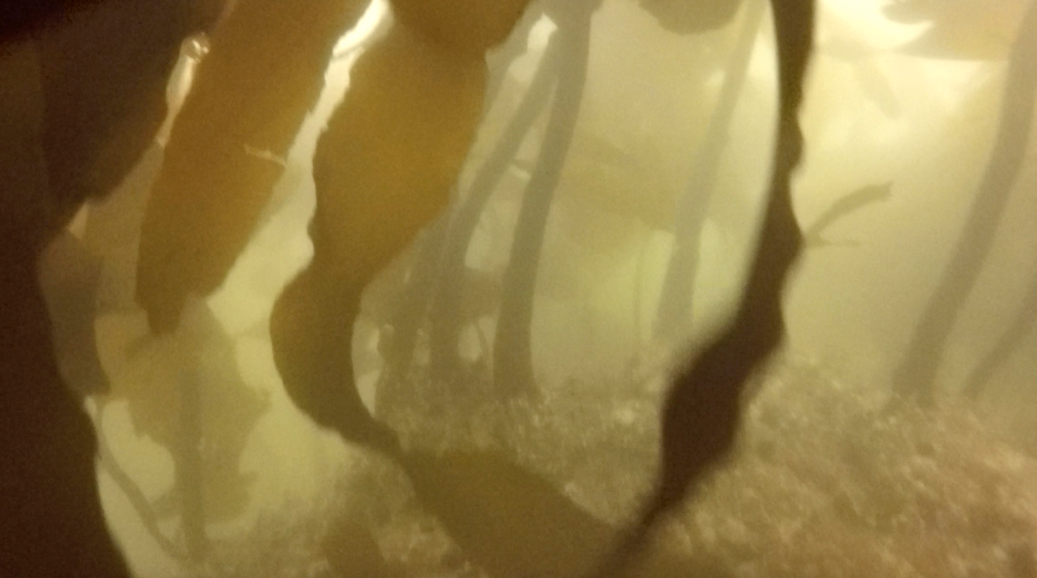
Figure 4. A gray whale surfaces in a large kelp bed during a foraging bout along the Oregon coast. (Source: GEMM Lab).
So, what does all of this information have to do with gray whales? Given their affinity for kelp habitats (Figure 4) and their zooplankton prey that aggregates there, changes to kelp ecosystems may affect gray whale health and ecology. This aspect of the complex kelp trophic web has not been examined to date; thus one of my PhD chapters focuses on the response of gray whales to changing kelp ecosystems along the southern Oregon coast. To do this, I am examining 6 years of data collected during the TOPAZ/JASPER project in Port Orford, to look at the relationships between kelp health, sea urchin density, zooplankton abundance, and gray whale foraging effort over space and time. Documenting impacts of changing kelp forests on gray whales is important to assist management efforts as healthy and abundant kelp seems critical in providing ample food opportunities for these iconic Pacific Northwest marine predators.
Did you enjoy this blog? Want to learn more about marine life, research, and conservation? Subscribe to our blog and get a weekly alert when we make a new post! Just add your name into the subscribe box on the left panel.
References
Bennett S, et al. The ‘Great Southern Reef’: Social, ecological and economic value of Australia’s neglected kelp forests. Marine and Freshwater Research 67:47-56.
Dayton PK (1985) Ecology of kelp communities. Annual Review of Ecology and Systematics 16:215-245.
Filbee-Dexter K, Scheibling RE (2014) Sea uechin barrens as alternative stable states of collapsed kelp ecosystems. Marine Ecology Progress Series 495:1-25.
Frölicher TL, Fischer EM, Gruber N (2018) Marine heatwaves under global warming. Nature 560:360-364.
Harvell CD, et al. (2019) Disease epidemic and a marine heat wave are associated with the continental-scale collapse of a pivotal predator (Pycnopodia helianthoides). Science Advances 5(1) doi:10.1126/sciadv.aau7042.
Krumhansl KA, et al. (2016) Global patterns of kelp forest change over the past half-century. Proceedings of the National Academy of Sciences of the United States of America 113(48):13785-13790.
Pinnegar JK, et al. (2000) Trophic cascades in benthic marine ecosystems: lessons for fisheries and protected-area management. Environmental Conservation 27:179-200.
Rogers-Bennett L, Catton CA (2019) Marine heat wave and multiple stressors tip bull kelp forest to sea urchin barrens. Scientific Reports 9:15050.
Sala E, Boudouresque CF, Harmelin-Vivien M (1998) Fishing, trophic cascades and the structure of algal assemblages; evaluation of an old but untested paradigm. Oikos 82:425-439.
Steneck RS, et al. (2002) Kelp forest ecosystems: biodiversity, stability, resilience and future. Environmental Conservation 29:436-459.
Tegner MJ, Dayton PK, Edwards PB, Riser KL (1996) Is there evidence for the long-term climatic change in southern California kelp forests? California Cooperative Oceanic Fisheries Investigations Report 37:111-126.
Torres LG, Nieukirk SL, Lemos L, Chandler TE (2018) Drone up! Quantifying whale behavior from a new perspective improves observational capacity. Frontiers in Marine Science doi:10.3389/fmars.2019.00319.
Dr. Alejandro A. Fernández Ajó, Postdoctoral Scholar, Marine Mammal Institute – OSU Department of Fisheries, Wildlife, & Conservation Sciences, Geospatial Ecology of Marine Megafauna (GEMM) Lab.
I often receive two reactions when asked what I am currently working on; one is “Wow! That is a very cool job, it must be amazing to work with such incredible animals!”, the other is “How do you do that and why is that important?”. So, today I decided to blog about some of the reasons why it is important to develop a pregnancy test for gray whales and how we are doing this.
In a previous blogpost, I described the many ways in which whales play critical roles in sustaining marine ecosystem. Briefly, whales can enhance marine productivity by vertically and horizontally mixing of ocean waters, promoting primary production, and mitigating climate change by sequestering carbon with their large biomass and long life-span (1-3). Even after they die, their carcasses can contribute to biodiversity creating new habitat on the seafloor (4). But, over several decades, the whaling industry drastically removed whales around the globe, with some species and populations depleted to near extinction (5). Consequently, these depleted whale populations now play a diminished role in ocean ecosystem processes and their recovery is currently challenged by an increasing number of modern anthropogenic impacts. Hence, working towards whale conservation is essential for keeping a healthy marine ecosystem.
Working and designing effective strategies for conservation biology often involves gaining knowledge regarding the reproductive parameters of individual animals in wild populations. This information is critical for understanding population trends and the underlaying mechanisms that affect animal welfare and their potential for recovery. However, getting such information from free-living whales can be challenging (see Hunt et al. 2013). While we know that whales typically have long life-spans, lengthy generation times, extended parental care, and high survival rates, detailed knowledge on the life history and general reproductive biology of free-ranging whales is limited for the majority of the whale populations. In fact, much of what we do know about whale reproduction is derived from whaling records. Only recently, conservation physiology approaches (see our previous post here) have contributed alternative and non-invasive methods for monitoring key physiological processes that can help monitor a whale’s reproductive biology and determine reproductive parameters such as sexual maturity and pregnancy (6-9).
In this clip you can see an example of a fecal sample collection from a gray whale off the Oregon coast. We can look at hormones in the fecal samples which are useful indicators for endocrine assessments of free-swimming whales. Fecal sample and footage filmed under NOAA/NMFS permit #16111.
Gray whales (Eschrichtius robustus) in the Eastern North Pacific (ENP) typically undertake annual migrations between their lower latitude breeding grounds in the coastal waters of the Baja California Peninsula, Mexico, and the foraging grounds located on the Bering and Chukchi Seas (10). However, among the ENP whales a distinct subgroup of about 230 whales shorten their migration to feed in the coastal waters of Northern California, Oregon, and southeastern Alaska (11). This group of whales is known as the gray whale Pacific Coast Feeding Group (PCFG).
Since 2016, the GEMM Lab has monitored individual gray whales within the PCFG off the Oregon coast (check the GRANITE project). Gray whales have a distinct mottled skin; and each individual whale presents a unique pigmentation pattern that allows for the individual identification of whales. We can identify who is who among the whales who visit the Oregon coast. In this way, we can keep a detailed record of re-sightings of known individuals (visit our new web site to know more about the lives of individual whales that visit the Oregon coast). We have high individual re-sighting rates, so this unique opportunity helps us keep a long-term data series for individual whales to monitor their health, body condition, and reproductive status over time, and thus further develop and advance our non-invasive study methods.
We are combining behavioral and feeding ecology with drone photogrammetry and endocrinology of the same individual whales to help us understand the relationships between natural and anthropogenic drivers with biological parameters. In this way, following individual whales, we are developing sensitive biomarkers to monitor and infer about the population health, population trends, and identify stressors that impact their recovery and welfare. In particular, we are now working to develop a noninvasive approach to detect pregnancy in gray whales based on fecal hormone analyses.
In this picture you can see “Rose”, a gray whale calf, on top of her mother “Scarlett”. Scarlett is one of the most recognizable whales from the PCFG, due to a large scar on the right side of her back (not visible in this picture). She has been observed along the Pacific NW coast since 1996, so she is at least 26 years old today. We know 3 of her calves. Following individual whales like Scarlett is helping us to better understand the gray whale reproductive biology. Photo by Alejandro Fernandez Ajo taken under NOAA/NMFS permit #21678.
In marine mammals, the progesterone hormone is secreted in the ovaries during the estrous cycle and gestation, and is the predominant hormone responsible for sustaining pregnancy (12). As the hormones are cleared from the blood into the gut, they are metabolized and eventually excreted in feces; fecal samples represent a cumulative and integrated concentration of hormone metabolites (13-14), which are useful indicators for endocrine assessments of free-swimming whales. Several studies show that changes in hormone concentration correlate in meaningful ways with exposure to stressors (15-16) and changes in reproductive status (17-19). We are using our long data series of fecal hormones and individual life histories to advance our understanding on the gray whales’ reproductive biology. We are close to developing a technique that will allow us to detect pregnancy in whales based in fecal hormones analyses and photogrammetry. Stay tuned for results from this pregnancy test!
Did you enjoy this blog? Want to learn more about marine life, research, and conservation? Subscribe to our blog and get a weekly alert when we make a new post! Just add your name into the subscribe box on the left panel.
References:
1- Pershing AJ, Christensen LB, Record NR, Sherwood GD, Stetson PB (2010) The impact of whaling on the ocean carbon cycle: Why bigger was better. PLoS ONE 5(8): e12444.
2- Roman J and McCarthy JJ. 2010. The whale pump: marine mammals enhance primary productivity in a coastal basin. PLoS ONE. 5(10): e13255.
3- Morissette L, Kaschner K, and Gerber LR. 2010. “Whales eat fish”? Demystifying the myth in the Caribbean marine ecosystem. Fish Fish 11: 388–404.
4- Smith CR, Roman J, Nation JB. A metapopulation model for whale-fall specialists: The largest whales are essential to prevent species extinctions. J. Mar. Res. 77, 283–302 (2019).
5- Branch TA, Williams TM. Legacy of industrial whaling. Whales. Whal. Ocean Ecosyst. 2006, 262–278 (2006).
6- Kellar NM, Keliher J, Trego ML, Catelani KN, Hanns C, George JC, et al. Variation of bowhead whale progesterone concentrations across demographic groups and sample matrices. Endanger Species Res 2013; 22:61–72. https://doi.org/10.3354/esr00537.
7- Pallin L, Robbins J, Kellar N, Berube M, Friedlaender A. Validation of a blubber-based endocrine pregnancy test for humpback whales. Conserv Physiol 2018;6:1 11. https://doi.org/10.1093/conphys/coy031PMID:29942518.
8-Hunt KE, Robbins J, Buck CL, Bérubé M, Rolland RM (2019) Evaluation of fecal hormones for noninvasive research on reproduction and stress in humpback whales (Megaptera novaeangliae). Gen Comp Endocrinol 280: 24–34.
9-Melica, V., Atkinson, S., Calambokidis, J., Lang, A., Scordino, J., & Mueter, F. (2021). Application of endocrine biomarkers to update information on reproductive physiology in gray whale (Eschrichtius robustus). Plos one, 16(8), e0255368.
10-Swartz SL. Gray Whale. In: Wursig B, Thewissen JGM, Kovacs KM, editors. Encyclopedia of Marine Mammals (Third Edition). Elsevier;2018,p. 422–8.https://doi.org/10.1016/B978-0-12-804327-1.00140–0.
11-Calambokidis J, Darling JD, Deecke V, Gearin P, Gosho M, Megill W, et al. Abundance, range and movements of a feeding aggregation of gray whales (Eschrichtius robustus) from California to south-eastern Alaska in 1998. J Cetacean Res Manag 2002;4:267–76.
12- Bronson, F. H. (1989). Mammalian reproductive biology. University of Chicago Press.
13-Wasser SK, Hunt KE, Brown JL, Cooper K, Crockett CM, Bechert U, Millspaugh JJ, Larson S, Monfort SL (2000) A generalized fecal glucocorticoid assay for use in a diverse array of nondomestic mammalian and avian species. Gen Comp Endocrinol120:260–275.
14- Hunt, K.E., Rolland, R.M., Kraus, S.D., Wasser, S.K., 2006. Analysis of fecal glucocorticoids in the North Atlantic right whale (Eubalaena glacialis). Gen. Comp. Endocrinol. 148, 260–272. https://doi.org/10.1016/j.ygcen.2006.03.01215.
15- Lemos, L.S., Olsen, A., Smith, A., Burnett, J.D., Chandler, T.E., Larson, S., Hunt, K.E., Torres, L.G., 2021. Stressed and slim or relaxed and chubby? A simultaneous assessment of gray whale body condition and hormone variability. Mar. Mammal Sci. 1–11. https://doi.org/10.1111/mms.12877
16- Rolland, R., McLellan, W., Moore, M., Harms, C., Burgess, E., Hunt, K., 2017. Fecal glucocorticoids and anthropogenic injury and mortality in North Atlantic right whales Eubalaena glacialis. Endanger. Species Res. 34, 417–429. https://doi.org/10.3354/esr00866.
17-Rolland, R.M., Hunt, K.E., Kraus, S.D., Wasser, S.K., 2005. Assessing reproductive status of right whales (Eubalaena glacialis) using fecal hormone metabolites. Gen. Comp. Endocrinol. 142, 308–317. https://doi.org/10.1016/j.ygcen.2005.02.002
18- Valenzuela Molina M, Atkinson S, Mashburn K, Gendron D, Brownell RL. Fecal steroid hormones reveal reproductive state in female blue whales sampled in the Gulf of California, Mexico. Gen Comp Endocrinol 2018;261:127–35.https://doi.org/10.1016/j.ygcen.2018.02.015 PMID:29476760.
19- Hunt, K. E., Robbins, J., Buck, C. L., Bérubé, M., & Rolland, R. M. (2019). Evaluation of fecal hormones for noninvasive research on reproduction and stress in humpback whales (Megaptera novaeangliae). General and Comparative Endocrinology, 280, 24-34.
When I wrote my first blog on individual specialization well over a year ago, I just skimmed the surface of the literature on this topic and only started to recognize the importance of studying individual specialization. The question, “is there individual specialization in the PCFG of gray whales?” is the focus of my first thesis chapter and the results will affect all my subsequent work. Therefore, the literature and concepts of individual specialization are a focus of my literature review and studies.
In my previous blog I focused on common characteristics of individuals that are similarly specialized as an underlying driver of individual specialization. While these characteristics (often attributable to age, sex, or physical traits) are important to consider, I’ve learned that the list of drivers of individual specialization is long and that many variables are dynamic. Of all the drivers I’ve learned about, competition is among the most common.
Competition is a major driver of individual specialization, and a common driver of competition is resource availability. When resource availability decreases, whether caused by increasing population density or changing environmental conditions, competition for that resource increases. As competition increases, individuals have a choice. They can choose to engage in competition, either by racing, fighting, or sharing [1], which can be costly, or they can diffuse the competition by focusing on a different resource. This second approach would be considered niche partitioning in the prey dimension. Niche partitioning is a way for individuals to share ecological space by using different resources. Essentially, individuals can share habitat without having to engage in direct competition by pursuing different prey types [2].
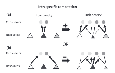
This switch to different prey types can change the degree of individual specialization present in the population (Figure 1). But the direction of the change is not constant. If all individuals were pursuing the same prey type under low competition conditions but then switched to different alternate prey types under high competition, then individual specialization would increase (Figure 1a). This direction has been observed across a range of species including sharks [3], otters [4]–[7], dolphins [8], [9], stickleback fish [10], [11], largemouth bass [12], banded mongoose [13], fur seals [14], and baleen whales [15].
However, if individuals were pursuing different prey types under low competition conditions (maybe because of underlying differences such as age or sex) but then switched to the same alternate prey types under high competition, diet overlap would increase, and individual specialization would decrease (Figure 1b). Furthermore, an individual might not switch to an entirely new prey type but instead add prey items to its diet [16]. This diet expansion under competition would also decrease individual specialization. Fewer studies have reported this direction but it’s been found in the common bumblebee [17] and in several neotropical vertebrate species [18], [19].
Figure `1. Figure 3 from Araújo et al. 2011 [20]. Illustration of how ecological mechanisms may affect the degree of individual specialization. Arrows linking resources to individual consumers indicate resource consumption (relative thickness indicates proportional contribution). Horizontal arrows indicate the sign (positive or negative) of the effect on the degree of individual specialization. (a) Consumers share the same preferred resource (dark gray tangle) but have different alternative resources (white and light gray triangles). As the preferred resource becomes scarce, consumers switch to different alternatives, increasing the degree of individual specialization. (b) Alternatively, consumers have distinct preferred resources, so that as resources become scarce, individuals converge to the alternative resource (dark gray triangle), reducing diet variation.
Interestingly, its hypothesized that individual specialization driven by competition is one of the factors that facilitates the formation and existence of stable groups [21]. For example, a study on resident female dolphins in Sarasota Bay, FL, USA found that females with high spatial overlap used distinct foraging specializations [8](Figure 2). This study illustrates how partitioning prey enabled spatial and social coexistence. A study on banded mongooses reached a similar conclusion [13]. They found that specialization was highest in the biggest groups (with the most competition) and not explained by sex, age, or other inherent differences. They hypothesized that specialization increasing with competition reduced conflict and allowed the groups to remain stable. This study also highlighted the role of learning to determine an individual’s specialization.
Figure 2. A bottlenose dolphin. Source: https://sarasotadolphin.org
Learning drives the distribution of knowledge throughout a population, which can lead to either specialization or generalization. ‘One-to-one’ learning, where one individual learns from one demonstrator, tends to promote individual specialization [21]. This form of transmission drives specialization because the individuals who learn the specialization tend to then carry on using, and eventually teaching, that specialization [6]. A common example of ‘one-to-one’ learning is vertical transmission from parent to offspring. It has been shown to transmit specializations in dolphins [22] and otters [6]. ‘One-to-one’ learning can occur outside of parent-offspring pairs; non-parent-offspring ‘one-to-one’ learning has been shown to drive specialization in banded mongooses [13](Figure 3).
However, other forms of social learning can promote more generalized foraging strategies. ‘Many-to-one’ or ‘one-to-many’ learning can reduce the presence of specialization in species [13], [21] as can the presence of conformity in a group [23], [24].
Figure 3. A group of banded mongooses. Source: http://socialisresearch.org/about-the-banded-mongoose-project/
The multiple drivers of specialization and their dynamic quality means that it is important to contextualize specialization. For example, a study on four species of neotropical frogs found varying degrees of specialization across multiple populations of each species [18]. The degree of specialization was dependent on a variety of drivers including predation and both intra- and inter-specific competition. Notably, the direction of the relationship between degree of specialization and each driver was species specific. This study highlights that one species may not always be more specialized than another, but that a populations’ specialization is context dependent.
Therefore, it is important to not only be aware of the degree of specialization present in a population, but to also understand its dynamics and drivers. These relationships can then be used to understand how, and why, a population may react to competition from other species, predators, and changes in resource availability [20]. A population’s specialization can also affect the specialization of other populations and community dynamics [25], therefore, it’s important to consider and study individual specialization on both the population and community level. I am excited to start using our incredible six-year dataset to start investigating these questions for PCFG gray whales, so stay tuned for results!
Did you enjoy this blog? Want to learn more about marine life, research, and conservation? Subscribe to our blog and get a weekly alert when we make a new post! Just add your name into the subscribe box on the left panel.
References
[1] M. Taborsky, M. A. Cant, and J. Komdeur, The Evolution of Social Behaviour. Cambridge: Cambridge University Press, 2021. doi: 10.1017/9780511894794.
[2] E. R. Pianka, “Niche Overlap and Diffuse Competition,” vol. 71, no. 5, pp. 2141–2145, 1974.
[3] P. Matich et al., “Ecological niche partitioning within a large predator guild in a nutrient-limited estuary,” Limnol. Oceanogr., vol. 62, no. 3, pp. 934–953, 2017, doi: https://doi.org/10.1002/lno.10477.
[4] S. D. Newsome et al., “The interaction of intraspecific competition and habitat on individual diet specialization: a near range-wide examination of sea otters,” Oecologia, vol. 178, no. 1, pp. 45–59, May 2015, doi: 10.1007/s00442-015-3223-8.
[5] M. T. Tinker, G. Bentall, and J. A. Estes, “Food limitation leads to behavioral diversification and dietary specialization in sea otters,” Proc. Natl. Acad. Sci., vol. 105, no. 2, pp. 560–565, Jan. 2008, doi: 10.1073/pnas.0709263105.
[6] M. T. Tinker, M. Mangel, and J. A. Estes, “Learning to be different: acquired skills, social learning, frequency dependence, and environmental variation can cause behaviourally mediated foraging specializations,” Evol. Ecol. Res., vol. 11, pp. 841–869, 2009.
[7] M. T. Tinker et al., “Structure and mechanism of diet specialisation: testing models of individual variation in resource use with sea otters,” Ecol. Lett., vol. 15, no. 5, pp. 475–483, 2012, doi: 10.1111/j.1461-0248.2012.01760.x.
[8] S. Rossman et al., “Foraging habits in a generalist predator: Sex and age influence habitat selection and resource use among bottlenose dolphins (Tursiops truncatus),” Mar. Mammal Sci., vol. 31, no. 1, pp. 155–168, 2015, doi: https://doi.org/10.1111/mms.12143.
[9] L. G. Torres, “A kaleidoscope of mammal , bird and fish : habitat use patterns of top predators and their prey in Florida Bay,” vol. 375, pp. 289–304, 2009, doi: 10.3354/meps07743.
[10] M. S. Araújo et al., “Network Analysis Reveals Contrasting Effects of Intraspecific Competition on Individual Vs. Population Diets,” Ecology, vol. 89, no. 7, pp. 1981–1993, 2008, doi: 10.1890/07-0630.1.
[11] R. Svanbäck and D. I. Bolnick, “Intraspecific competition drives increased resource use diversity within a natural population,” Proc. R. Soc. B Biol. Sci., vol. 274, no. 1611, pp. 839–844, Mar. 2007, doi: 10.1098/rspb.2006.0198.
[12] D. E. Schindler, J. R. Hodgson, and J. F. Kitchell, “Density-dependent changes in individual foraging specialization of largemouth bass,” Oecologia, vol. 110, no. 4, pp. 592–600, May 1997, doi: 10.1007/s004420050200.
[13] C. E. Sheppard et al., “Intragroup competition predicts individual foraging specialisation in a group-living mammal,” Ecol. Lett., vol. 21, no. 5, pp. 665–673, 2018, doi: 10.1111/ele.12933.
[14] L. Kernaléguen, J. P. Y. Arnould, C. Guinet, and Y. Cherel, “Determinants of individual foraging specialization in large marine vertebrates, the Antarctic and subantarctic fur seals,” J. Anim. Ecol., vol. 84, no. 4, pp. 1081–1091, 2015, doi: 10.1111/1365-2656.12347.
[15] E. M. Keen and K. M. Qualls, “Respiratory behaviors in sympatric rorqual whales: the influence of prey depth and implications for temporal access to prey,” J. Mammal., vol. 99, no. 1, pp. 27–40, Feb. 2018, doi: 10.1093/jmammal/gyx170.
[16] R. H. MacArthur and E. R. Pianka, “On Optimal Use of a Patchy Environment,” Am. Nat., vol. 100, no. 916, pp. 603–609, 1966, doi: 10.1086/282454.
[17] C. Fontaine, C. L. Collin, and I. Dajoz, “Generalist foraging of pollinators: diet expansion at high density,” J. Ecol., vol. 96, no. 5, pp. 1002–1010, 2008, doi: 10.1111/j.1365-2745.2008.01405.x.
[18] R. Costa-Pereira, V. H. W. Rudolf, F. L. Souza, and M. S. Araújo, “Drivers of individual niche variation in coexisting species,” J. Anim. Ecol., vol. 87, no. 5, pp. 1452–1464, 2018, doi: 10.1111/1365-2656.12879.
[19] M. M. Pires, P. R. Guimarães Jr, M. S. Araújo, A. A. Giaretta, J. C. L. Costa, and S. F. dos Reis, “The nested assembly of individual-resource networks,” J. Anim. Ecol., vol. 80, no. 4, pp. 896–903, 2011, doi: 10.1111/j.1365-2656.2011.01818.x.
[20] M. S. Araújo, D. I. Bolnick, and C. A. Layman, “The ecological causes of individual specialisation,”Ecol. Lett., vol. 14, no. 9, pp. 948–958, 2011, doi: https://doi.org/10.1111/j.1461-0248.2011.01662.x.
[21] C. E. Sheppard, R. Heaphy, M. A. Cant, and H. H. Marshall, “Individual foraging specialization in group-living species,” Anim. Behav., vol. 182, pp. 285–294, Dec. 2021, doi: 10.1016/j.anbehav.2021.10.011.
[22] S. Wild, S. J. Allen, M. Krützen, S. L. King, L. Gerber, and W. J. E. Hoppitt, “Multi-network-based diffusion analysis reveals vertical cultural transmission of sponge tool use within dolphin matrilines,” Biol. Lett., vol. 15, no. 7, p. 20190227, Jul. 2019, doi: 10.1098/rsbl.2019.0227.
[23] L. M. Aplin, D. R. Farine, J. Morand-Ferron, A. Cockburn, A. Thornton, and B. C. Sheldon, “Experimentally induced innovations lead to persistent culture via conformity in wild birds,” Nature, vol. 518, no. 7540, pp. 538–541, Feb. 2015, doi: 10.1038/nature13998.
[24] E. Van de Waal, C. Borgeaud, and A. Whiten, “Potent Social Learning and Conformity Shape a Wild Primate’s Foraging Decisions,” Science, Apr. 2013, doi: 10.1126/science.1232769.
[25] D. I. Bolnick et al., “Why intraspecific trait variation matters in community ecology,” Trends Ecol. Evol., vol. 26, no. 4, pp. 183–192, Apr. 2011, doi: 10.1016/j.tree.2011.01.009.
Dr. KC Bierlich, Postdoctoral Scholar, OSU Department of Fisheries, Wildlife, & Conservation Sciences, Geospatial Ecology of Marine Megafauna (GEMM) Lab
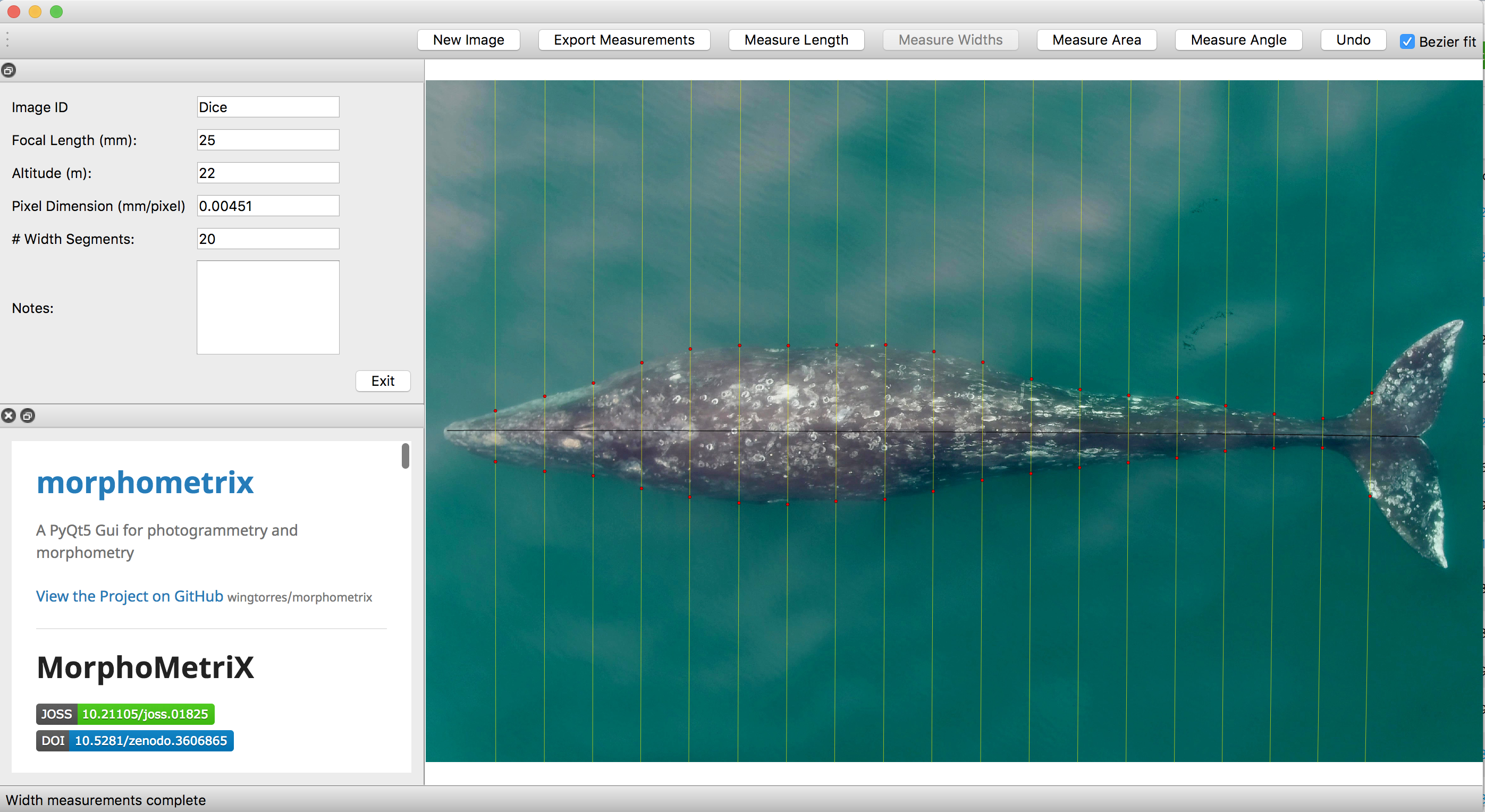
In my last blog, I discussed how to obtain morphological measurements from drone-based imagery of whales and the importance of calculating and considering uncertainty, as different drone platforms have varying levels of measurement uncertainty. But how does uncertainty scale and propagate when multiple measurements are combined, such as when measuring body condition of the whole animal? In this blog, I will discuss the different methods used for measuring body condition of baleen whales from drone-based imagery and how uncertainty differs between these metrics.
Body condition is defined as the energy stored in the body as a result of feeding and is assumed to indicate an animal’s overall health, as it reflects the balance between energy intake and investment toward growth, maintenance and reproduction (Peig and Green, 2009). Thus, body condition reflects the foraging success of an individual, as well as the potential for reproductive output and the quality of habitat. For example, female North American brown bears (Ursus arctos) in high quality habitats were in better body condition, produced larger litter sizes, and lived in greater population densities compared to females in lower quality habitats (Hilderbrand et al., 1999). As Dawn Barlow and Will Kennerley discussed in their recent blog, baleen whales are top predators and serve as ecosystem sentinels that shed light not only on the health of their population, but on the health of their ecosystem. As ocean climate conditions continue to change, monitoring the body condition of baleen whales is important to provide insight on how their population and ecosystem is responding.
As discussed in a previous blog, drones serve as a valuable tool for obtaining morphological measurements of baleen whales to estimate their body condition. Images are imported into photogrammetry software, such as MorphoMetriX (Torres and Bierlich, 2020), to measure the total length of an individual and that is then divided into perpendicular width segments (i.e., in 5 or 10% increments) down the body (Fig. 1). These total length and width measurements are then used to estimate body condition in either 1-, 2-, or 3-dimensions: a single width (1D), a projected dorsal surface area (2D), or a body volume measure (3D). These 1D, 2D, and 3D measurements of body condition can then be standardized by total length to produce a relative measure of an individual’s body condition to compare among individuals and populations.
Figure 1. An example of a Pacific Coast Feeding Group (PCFG) gray whale measured in MorphoMetriX (Torres & Bierlich, 2020).
While several different studies have used each of these dimensions to assess whale body condition, it is unclear how these measurements compare amongst each other. Importantly, it is also unclear how measurement uncertainty scales across these multiple dimensions and influences inference, which can lead to misinterpretation of data. For example, the surface area and volume of two geometrically similar bodies of different sizes are not related to their linear dimensions in the same ratio, but rather to the second and third power, respectively (i.e., x2 vs. x3). Similarly, uncertainty should not be expected to scale linearly across 1D, 2D, and 3D body condition measurements.
The second chapter of my dissertation, which was recently published in Frontiers in Marine Science and includes Clara Bird and Leigh Torres as co-authors, compared the uncertainty associated with 1D, 2D, and 3D drone-based body condition measurements in three baleen whale species with different ranges in body sizes: blue, humpback, and Antarctic minke whales (Figure 2) (Bierlich et al., 2021). We used the same Bayesian model discussed in my last blog, to incorporate uncertainty associated with each 1D, 2D, and 3D estimate of body condition.
Figure 2. An example of total length and perpendicular width (in 5% increments of total length) measurements of an individual blue, humpback and Antarctic minke whale. Each image measured using MorphoMetriX (Torres and Bierlich, 2020).
We found that uncertainty does not scale linearly across multi-dimensional measurements, with 2D and 3D uncertainty increasing by a factor of 1.45 and 1.76 compared to 1D, respectively. This result means that there is an added cost of increased uncertainty when utilizing a multidimensional body condition measurement. Our finding is important to help researchers decide which body condition measurement best suits their scientific question, particularly when using a drone platform that is susceptible to greater error – as discussed in my previous blog. However, a 1D measurement only relies on a single width measurement, which may be excluding other regions of an individual’s body condition that is important for energy storage. In these situations, a 2D or 3D measure may be more appropriate.
We found that when comparing relative measures of body condition (standardized by total length of the individual), each standardized metric was highly correlated with one another. This finding suggests that 1D, 2D, and 3D metrics will draw similar relative predictions of body condition for individuals, allowing researchers to be confident they will draw similar conclusions relating to the body condition of individuals, regardless of which standardized metric they use. However, when comparing the precision of each of these metrics, the body area index (BAI) – a 2D standardized metric – displayed the highest level of precision. This result highlights how BAI can advantageously detect small changes in body condition, which is useful for comparing individuals or even tracking the same individual over time.
BAI was developed by the GEMM Lab (Burnett et al., 2018) and was designed to be similar to body mass index (BMI) in humans [BMI = mass (kg)/(height (m))2], where BAI uses the calculated surface area as a surrogate for body mass. In humans, a healthy BMI range is generally considered 18.5–24.9, below 18.5 is considered underweight, above 24.9 is considered overweight, and above 30 is considered obese (Flegal et al., 2012). Identifying a healthy range in BAI for baleen whales is challenged by a limited knowledge of what a “healthy” body condition range is for a whale. We found strong evidence that a healthy range of BAI is species-specific, as each species displayed a distinctive range in BAI: blue whales: 11–16; AMW: 17–24; humpback whales: 23–32; humpback whale calves: 23–28 (Fig. 3). These differences in BAI ranges likely reflect differences in the body shape of each species (Fig. 4). For example, humpbacks have the widest range of BAI compared to these other two species, which was also reflected in their larger variation in perpendicular widths (Figs. 2-4). Thus, it seems that BAI offers conditionally “scalefree” comparisons between species, yet it is unreasonable to set a single, all-whale BAI threshold to determine “healthy” versus “unhealthy” body condition. Collecting a large sample of body condition measurements across many individuals and demographic units over space and time with information on vital rates (e.g., reproductive capacity) will help elucidate a healthy BAI range for each species.
Figure 3. Body area index (BAI) for each species. AMW = Antarctic minke whale. Figure from Bierlich et al. (2021).Figure 4. A) Absolute widths (m) and B) relative widths, standardized by total length (TL) to help elucidate the different body shapes of Antarctic minke whales (AMW; n = 40), blue whales (n = 32), humpback whales (n = 40), and humpback whale calves (n = 15). Note how the peak in body width occurs at a different percent body width between species, demonstrating the natural variation in body shape between baleen whales. Figure from Bierlich et al. (2021).
Over the past six years, the GEMM Lab has been collecting drone images of Pacific Coast Feeding Group (PCFG) gray whales off the coast of Oregon to measure their BAI (see GRANITE Project blog). Many of the individuals we encounter are seen across years and throughout the foraging season, providing an opportunity to evaluate how an individual’s BAI is influenced by environmental variation, stress levels, maturity, and reproduction. These data will in turn help determine what the healthy range in BAI for gray whales is. For example, linking BAI to pregnancy – whether a whale is currently pregnant or becomes pregnant the following season – will help determine what BAI is needed to support calf production. We are currently analyzing hundreds of body condition measurements from 2016 – 2021, so stay tuned for upcoming results!
References
Bierlich, K. C., Hewitt, J., Bird, C. N., Schick, R. S., Friedlaender, A., Torres, L. G., … & Johnston, D. W. (2021). Comparing Uncertainty Associated With 1-, 2-, and 3D Aerial Photogrammetry-Based Body Condition Measurements of Baleen Whales. Frontiers in Marine Science, 1729.
Burnett, J. D., Lemos, L., Barlow, D., Wing, M. G., Chandler, T., & Torres, L. G. (2018). Estimating morphometric attributes of baleen whales with photogrammetry from small UASs: A case study with blue and gray whales. Marine Mammal Science, 35(1), 108–139.
Flegal, K. M., Carroll, M. D., Kit, B. K., & Ogden, C. L. (2012). Prevalence of Obesity and Trends in the Distribution of Body Mass Index Among US Adults, 1999-2010. JAMA, 307(5), 491. https://doi.org/10.1001/jama.2012.39
Hilderbrand, G. V, Schwartz, C. C., Robbins, C. T., Jacoby, M. E., Hanley, T. A., Arthur, S. M., & Servheen, C. (1999). The importance of meat, particularly salmon, to body size, population productivity, and conservation of North American brown bears. Canadian Journal of Zoology, 77(1), 132–138.
Peig, J., & Green, A. J. (2009). New perspectives for estimating body condition from mass/length data: the scaled mass index as an alternative method. Oikos, 118(12), 1883–1891.
Torres, W., & Bierlich, K. C. (2020). MorphoMetriX: a photogrammetric measurement GUI for morphometric analysis of megafauna. Journal of Open Source Software, 5(45), 1825–1826.