Return of the whales: The GRANITE 2022 field season comes to a close

Clara Bird, PhD Candidate, OSU Department of Fisheries, Wildlife, and Conservation Sciences, Geospatial Ecology of Marine Megafauna Lab

It’s hard to believe that it’s already been four and half months since we started the field season (check out Lisa’s blog for a recap of where we began), but as of this weekend the GRANITE project’s 8th field season has officially ended! As the gray whales wrap up their foraging season and start heading south for the winter, it’s time for us to put our gear into storage, settle into a new academic year, and start processing the data we spent so much time collecting.

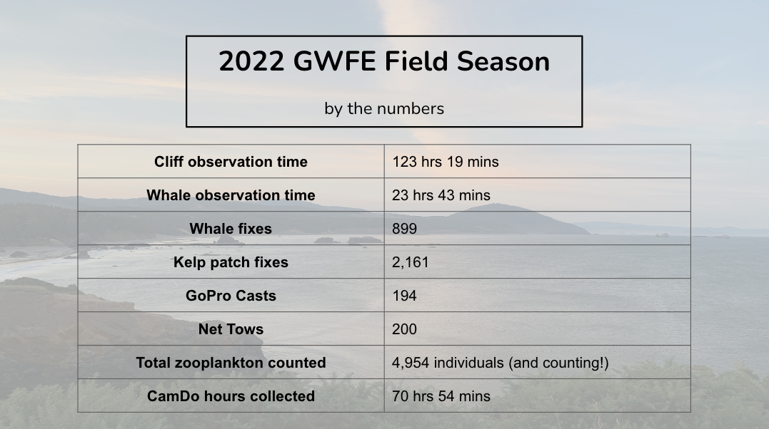
The field season can be quite an intense time (40 days equaling over 255 hours on the water!), so we often don’t take a moment to reflect until the end. But this season has been nothing short of remarkable. As you may remember from past blogs, the past couple years (2020-21) have been a bit concerning, with lower whale numbers than previously observed. Since many of us started working on the project during this time, most of us were expecting another similar season. But we were wrong in the best way. From the very first day, we saw more whales than in previous years and we identified whales from our catalog that we hadn’t seen in several years.

Image 1: Collage of photos from our field season.

We identified friends – old and new!

This season we had 224 sightings of 63 individual whales. Of those 63, 51 were whales from our catalog (meaning we have seen them in a previous season). Of these 51 known whales, we only saw 20 of them last year! This observation brings up interesting questions such as, where did most of these whales forage last year? Why did they return to this area this year? And, the classic end of season question, what’s going to happen next year?

We also identified 12 whales that were not in our catalog, making them new to the GEMM lab. Two of our new whales are extra exciting because they are not just new to us but new to the population; we saw two calves this year! We were fortunate enough to observe two mom-calf pairs in July. One pair was of a “new” mom in our catalog and her calf. We nicknamed this calf “Roly-poly” because when we found this mom-calf pair, we recorded some incredible drone footage of “roly-poly” continuously performing body rolls while their mom was feeding nearby (video 1). 

Video 1: “Roly-poly” body rolling while their mom headstands. NOAA/NMFS permit #21678.

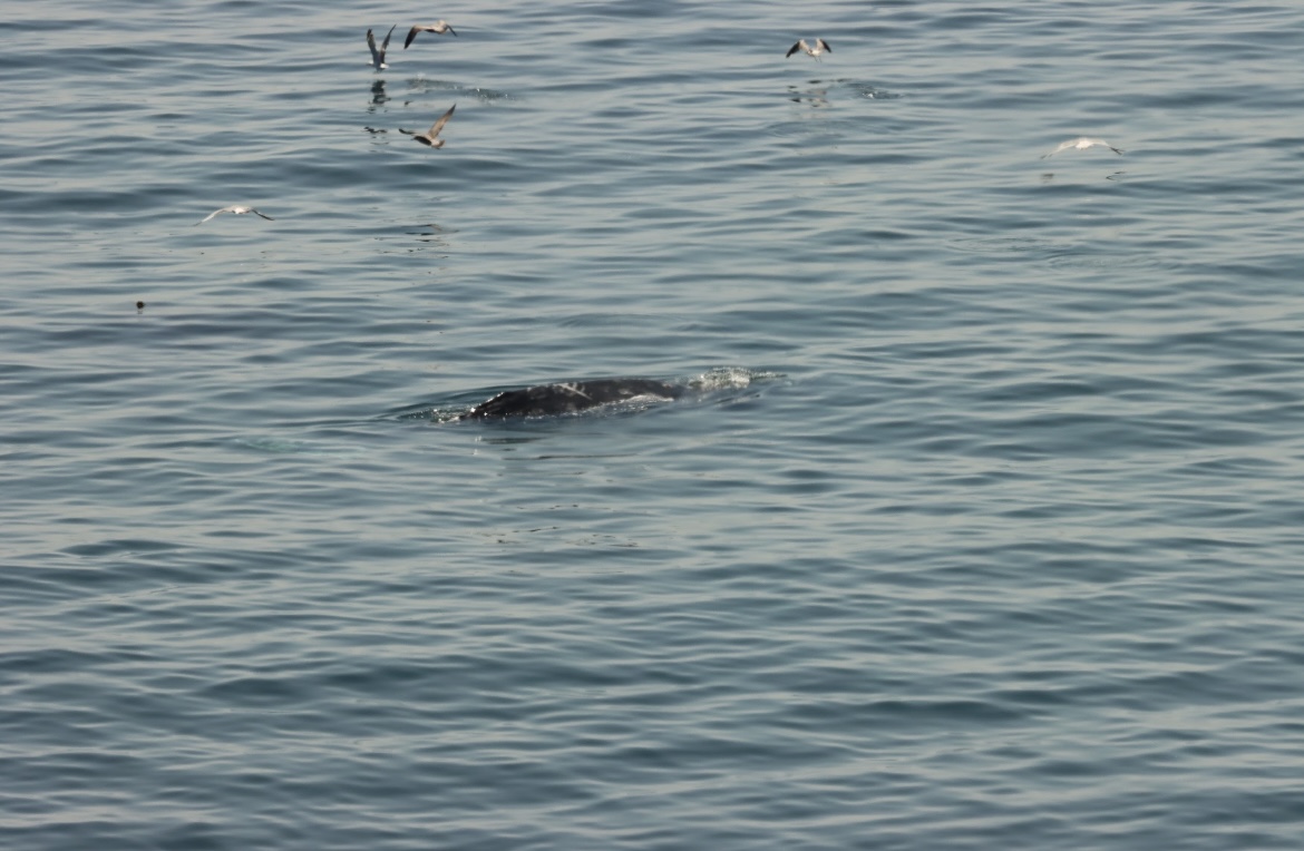
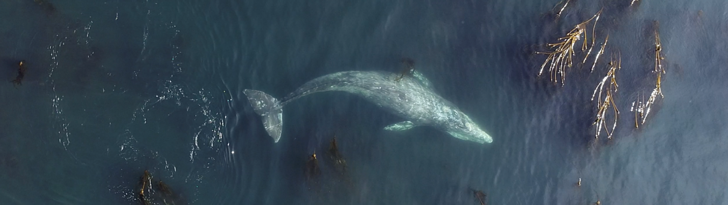
The other pair includes a known GEMM lab whale, Luna, and her calf (currently nicknamed “Lunita”). We recently found “Lunita” feeding on their own in early October (Image 2), meaning that they are now independent from its mom (for more on mom-calf behavior check out Celest’s recent blog). We’ll definitely be on the lookout for Roly-Poly and Lunita next year!

Image 2: (left) drone image of Luna and Lunita together in July and (right) drone image of Lunita on their own in October.  NOAA/NMFS permit #21678.

We flew, we scooped, we collected heaps of data!

From our previous blogs you probably know that in addition to photo-ID images, our other two most important forms of data collection are drone flights (for body condition and behavior data) and fecal samples (for hormone analysis). And this season was a success for both! 

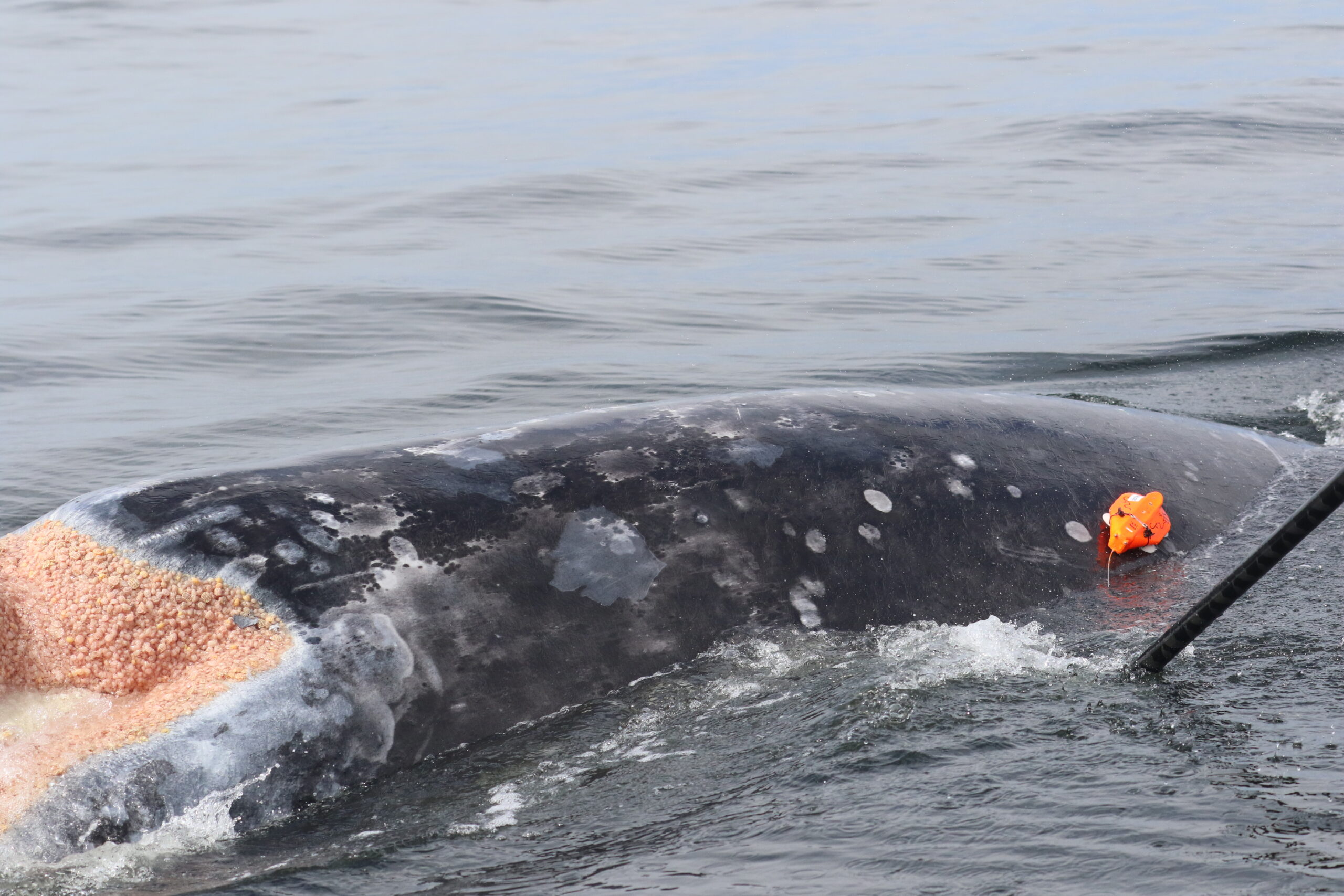
We conducted 124 flights over 49 individual whales. The star of these flights was a local favorite Scarlett who we flew over 18 different times. These repeat samples are crucial data for us because we use them to gain insight into how an individual’s body condition changes throughout the season. We also recorded loads of behavior data, collecting footage of different foraging tactics like headstanding, side-swimming, and surfacing feeding on porcelain crab larvae (video 2)!

Video 2: Two whales surface feeding on porcelain crab larvae. NOAA/NMFS permit #21678.

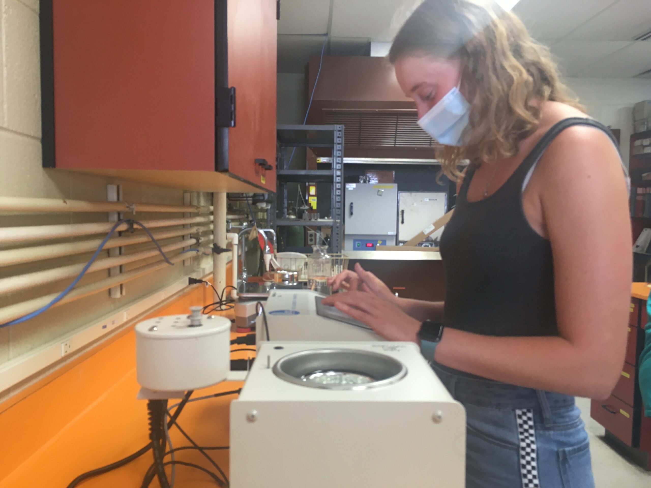
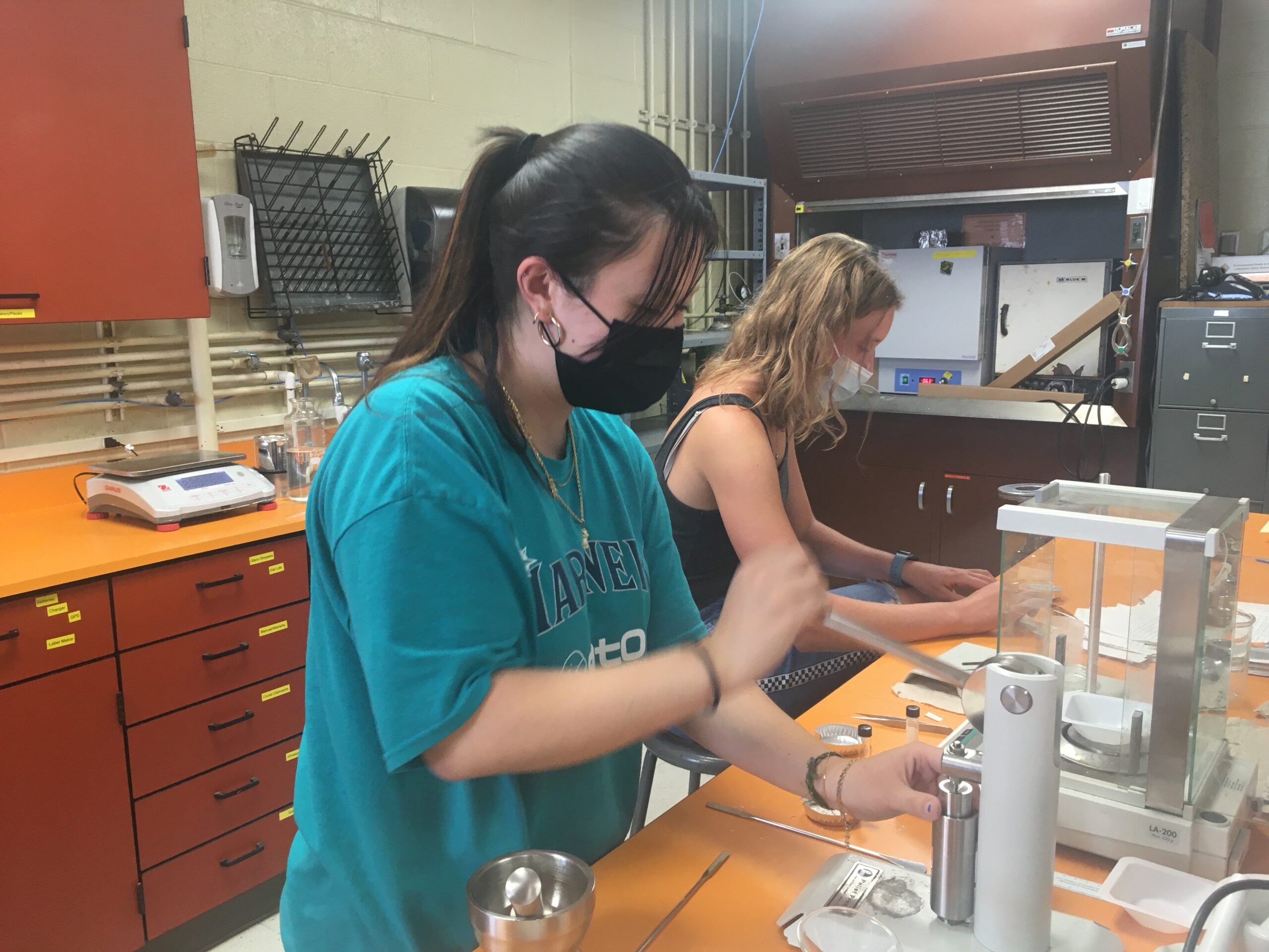
We also collected 61 fecal samples from 26 individual whales (Image 3). The stars of that dataset were Soléand Peak who tied with 7 samples each. These hard-earned samples provide invaluable insight into the physiology and stress levels of these individuals and are a crucial dataset for the project.

Image 3: Photos of fecal sample collection. Left – a very heavy sample, center: Lisa and Enrico after collecting the first fecal sample of the season, right: Clara and Lisa celebrating a good fecal sample collection.

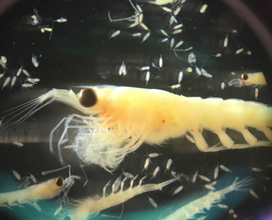
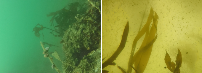
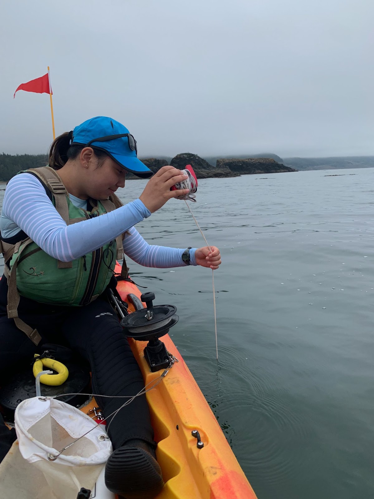
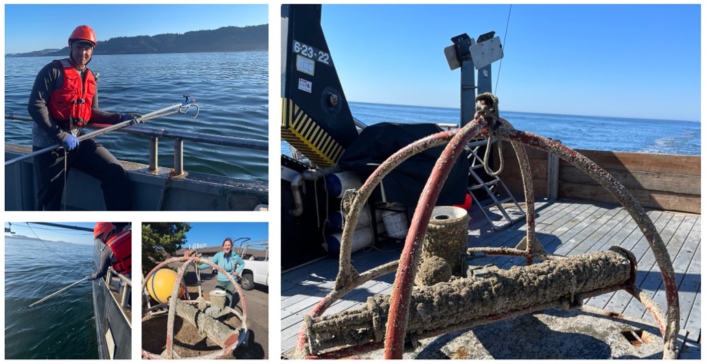
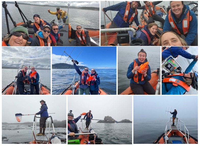
On top of all that amazing data collection we also collected acoustic data with our hydrophones, prey data from net tows, and biologging data from our tagging efforts. Our hydrophones were in the water all summer recording the sounds that the whales are exposed to, and they were successfully recovered just a few weeks ago (Image 4)! We also conducted 69 net tows to sample the prey near where the whales were feeding and identify which prey the whales might be eating (Image 5). Lastly, we had two very successful tagging weeks during which we deployed (and recovered!) a total of 9 tags, which collected over 30 hours of data (Image 6; check out Kate’s blog for more on that).

Image 4 – Photos from hydrophone recovery.
Image 5: Photos from zooplankton sampling.
Image 6: Collage of photos from our two tagging efforts this season.

Final thoughts

All in all, it’s been an incredible season. We’ve seen the return of old friends, collected lots of awesome data, and had some record-breaking days (28 whales in one day!). As we look toward the analysis phase of the year, we’re excited to dig into our eight-year dataset and work to understand what might explain the increase in whales this year.

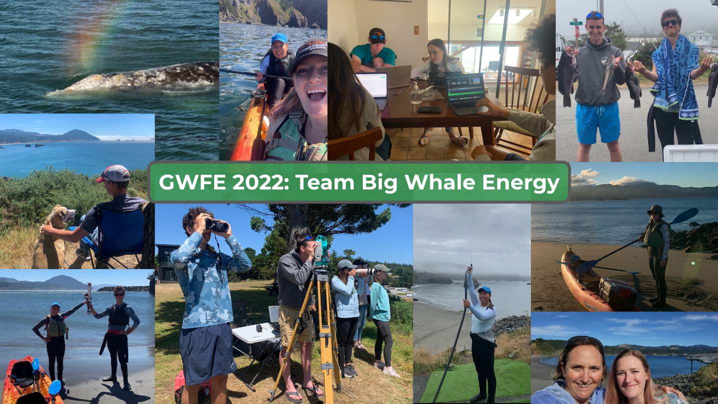
To end on a personal note, looking through photos to put in this blog was the loveliest trip down memory lane (even though it only ended a few days ago) – I am so honored and proud to be a part of this team. The work we do is hard; we spend long hours on a small boat together and it can be a bit grueling at times. But, when I think back on this season, my first thoughts are not of the times I felt exhausted or grumpy, but of all the joy we felt together. From the incredible whale encounters to the revitalizing snacks to the off-key sing alongs, there is no other team I would rather do this work with, and I so look forward to seeing what next season brings. Stay tuned for more updates from team GRANITE!

Did you enjoy this blog? Want to learn more about marine life, research, and conservation? Subscribe to our blog and get a weekly alert when we make a new post! Just add your name into the subscribe box below!

Loading

Bombs Away! A Summer of Bomb Calorimetry

By Hadley Robinson, undergraduate student, OSU College of Earth, Ocean, and Atmospheric Sciences and School of Language, Culture, and Society

My name is Hadley Robinson and I am a sophomore undergraduate at OSU, double majoring in Environmental Science and Spanish. This summer, I had the privilege of working with Rachel on her PhD research project involving bomb calorimetry, a technique that allows you to quantify the caloric content of organisms like the zooplankton krill.

Hadley preparing the bomb calorimetry machine to run a sample (photo by Rachel Kaplan).

Prior to this internship, I had never worked in a lab before, and as an environmental science major, I had no previous exposure to oceanography. The connection that Rachel made between our labwork and the broader goal of helping decrease whale entanglement events sparked my interest in this project. Our work this summer aimed to process a set of krill samples collected off the coast of Oregon and Washington, so that we could find the number of calories in single krill, and then look at patterns in krill caloric content based on their species, sex, and other characteristics. 

We first identified the krill by species and sex (this was my favorite part of the experiment!). I not only loved looking at them under the microscope, but I also loved how it became a collaborative process. We quickly began getting each other’s opinions on whether or not a krill was Euphausia pacifica, Thysanoessa spinifera, male, female, sexless, gravid (carrying eggs), and much more.

Female Thysanoessa spinifera krill (photo by Abby Tomita).

After identification, we weighed and dried the krill, and finally turned them into small pellets that could fit in an instrument called a bomb calorimeter. These pellets were placed individually into in a “bomb cell” that could then be filled with oxygen and receive a shock from a metal wire. When the machine sent an electric pulse through the wire and combusted the krill pellet, the water surrounding the bomb cell warmed very slightly. The instrument measures this minute temperature change and uses it to calculate the amount of energy in the combusted material. With this information, we were able to quantify how many calories each krill sample contained. Eventually, this data could be used to create a seasonal caloric map of the ocean. Assuming that foraging whales seek out regions with calorically dense prey, such a map could play a crucial role in predicting whale distributions. 

Working with Rachel taught me how dynamic the world of research really is. There were many variables that we had to control and factor into our process, such as the possibility of high-calorie lipids being lost if the samples became too warm during the identification process, the risk of a dried krill becoming rehumidified if it sat out in the open air, and even the tiny amount of krill powder inevitably lost in the pelletization process. This made me realize that we cannot control everything! Grappling with these realities taught me to think quickly, adapt, and most importantly, realize that it is okay to refine the process of research as it is being conducted. 

Intern Abby (left) pressing the krill powder into a pellet and Hadley (right) prepping the bomb (photo by Rachel Kaplan).

Did you enjoy this blog? Want to learn more about marine life, research, and conservation? Subscribe to our blog and get a weekly message when we post a new blog. Just add your name and email into the subscribe box below.

Loading

Putting Fitbits on whales: How tag data allows for estimating calories burned by foraging PCFG gray whales

By: Kate Colson, MSc Student, University of British Columbia, Institute for the Oceans and Fisheries, Marine Mammal Research Unit

Hello! My name is Kate Colson and I am a master’s student at the University of British Columbia, co-supervised by Dr. Andrew Trites of the Marine Mammal Research Unit and Dr. Leigh Torres of the GEMM Lab. As part of my thesis work, I have had the opportunity to spend the summer field season with Leigh and the GEMM Lab team. 

For my master’s I am studying the foraging energetics of Pacific Coast Feeding Group (PCFG) gray whales as part of the much larger Gray whale Response to Ambient Noise Informed by Technology and Ecology (GRANITE) project. Quantifying the energy expenditure of PCFG gray whales during foraging can help establish a baseline for how disturbance impacts the ability of this unique population to meet their energy needs. Additionally, determining how many calories are burned during different PCFG foraging behaviors might help explain why some gray whales are in better body condition than others.

To understand how much energy different PCFG foraging behaviors cost, I am using data from suction cup tags we have temporarily applied on PCFG gray whales (Figure 1). You can read more about the why the GEMM Lab started using these tags in an earlier blog here. What I want to talk about in this blog is how exactly we can use this tag data to estimate energy expenditure of PCFG gray whales. 

Figure 1. The famous “Scarlett” with a suction cup tag just attached using a carbon fiber pole (seen on far right). This minimally invasive tag has many data sensors, all of which sample at high frequencies, that can allow for an estimation of energy expenditure for different gray whale behaviors. Source: GEMM Lab; National Marine Fisheries Service (NMFS) permit no. 21678 

The suction cups tags used in this project have many data sensors that are useful for describing the movement of the tagged whale including accelerometers, magnetometers, gyroscopes, and pressure sensors, and all are sampling at high frequencies. For example, the accelerometer is taking 400 measurements per second! The accelerometer, magnetometer, and gyroscope take measurements in 3 dimensions along the X, Y, and Z-axes. The whale’s movement around the X-axis indicates roll (if the whale is swimming on its side), while movement around the Y-axis indicates pitch (if the whales head is oriented towards the surface or the sea floor). Changes in the whale’s movement around the Z-axis indicates if the whale is changing its swimming direction. Together, all of these sensors can describe the dive profile, body orientation, fluking behavior, and fine-scale body movements of the animal down to the second (Figure 2). This allows for the behavior of the tagged whale to be specifically described for the entirety of the tag deployment. 

Figure 2. An example of what the tag sensor data looks like. The top panels show the depth of the animal and can be used to determine the diving behavior of the whale. The middle panels show the body roll of the whale (the X axis) —a roll value close to 0 means the whale is swimming “normally” with no rotation to either side, while a higher roll value means the whale is positioned on its side. The bottom panels show the fluking behavior of the animal: each spike is the whale using its tail to propel itself through the water, with higher spikes indicating a stronger fluke stroke. Source: GEMM Lab, NMFS permit no. 21678

Although these suction cup tags are a great advancement in collecting fine-scale data, they do not have a sensor that actually measures the whale’s metabolism, or rate of calories burned by the whale. Thus, to use this fine-scale tag data as an estimate for energy expenditure, a summary metric must be calculated from the data and used as a proxy. The most common metric found in the literature is Overall Dynamic Body Acceleration (ODBA) and many papers have been published discussing the pros and cons of using ODBA as a proxy for energy expenditure (Brown et al., 2013; Gleiss et al., 2011; Halsey, 2017; Halsey et al., 2011; Wilson et al., 2020). The theory behind ODBA is that because an animal’s metabolic rate is primarily comprised of movement costs, then measuring the acceleration of the body is an effective way of determining energy expenditure. This theory might seem very abstract, but if you have ever worn a Fitbit or similar fitness tracking device to estimate how many calories you’ve burned during a workout, the same principle applies. Those fitness devices use accelerometers and other sensors, to measure the movement of your limbs and produce estimates of energy used. 

So now that we’ve established that the goal of my research is to essentially use these suction cup tags as Fitbits for PCFG gray whales, let’s look at how accelerometry data has been used to detect foraging behavior in large whales so far. Many accelerometry tagging studies have used rorquals as a focal species (see Shadwick et al. (2019) for a review). Well-known rorqual species include humpback, fin, and blue whales. These species forage by using lunges to bulk feed on dense prey patches in the water column. Foraging lunges are indicated by isolated periods of high acceleration that are easily detectable in the tag data (Figure 3; Cade et al., 2016; Izadi et al., 2022). 

Figure 3. Top image: A foraging blue whale performing a surface lunge (Photo credit: GEMM Lab). Note the dense aggregation of krill in the whale’s mouth. Bottom image: The signature acceleration signal for lunge feeding (adapted from Izadi et al., 2022). Each color represents one of the 3D axes of whale movement. The discrete periods of high acceleration represent lunges

However, gray whales feed very differently from rorquals. Gray whales primarily suction feed on the benthos, using their head to dig into the sediment and filter prey out of the mud using their baleen. Yet,  PCFG gray whales often perform many other foraging behaviors such as headstanding and side-swimming (Torres et al., 2018). Additionally, PCFG gray whales tend to feed in water depths that are often shallower than their body length. This shallow depth makes it difficult to isolate signals of foraging in the accelerometry data from random variation in the data and separate the tag data into periods of foraging behaviors (Figure 4).

Figure 4. Top image: A foraging PCFG gray whale rolls on its side to feed on mysid prey. Bottom image: The graph shows the accelerometry data from our suction cup tags that can be used to calculate Overall Dynamic Body Acceleration (ODBA) as a way to estimate energy expenditure. Each color represents a different axis in the 3D motion of the whale. The X-axis is the horizontal axis shows forward and backward movement of the whale, the Y-axis shows the side-to-side movement of the whale, and the Z-axis shows the up-down motion of the whale. Note how there are no clear periods of high acceleration in all 3 axes simultaneously to indicate different foraging behaviors like is apparent during lunges of rorqual whales. However, there is a pattern showing that when acceleration in the Z-axis (blue line) is positive, the X- and Y-axes (red and green lines) are negative. Source: GEMM Lab; NMSF permit no. 21678

But there is still hope! Thanks to the GEMM Lab’s previous work describing the foraging behavior of the PCFG sub-group using drone footage, and the video footage available from the suction cup tags deployed on PCFG gray whales, the body orientation calculated from the tag data can be a useful indication of foraging. Specifically, high body roll is apparent in many foraging behaviors known to be used by the PCFG, and when the tag data indicates that the PCFG gray whale is rolled onto its sides, lots of sediment (and sometimes even swarms of mysid prey) is seen in the tag video footage. Therefore, I am busy isolating these high roll events in the collected tag data to identify specific foraging events. 

My next steps after isolating all the roll events will be to use other variables such as duration of the roll event and body pitch (i.e., if the whales head is angled down), to define different foraging behaviors present in the tag data. Then, I will use the accelerometry data to quantify the energetic cost of performing these behaviors, perhaps using ODBA. Hopefully when I visit the GEMM Lab again next summer, I will be ready to share which foraging behavior leads to PCFG gray whales burning the most calories!

References

Brown, D. D., Kays, R., Wikelski, M., Wilson, R., & Klimley, A. P. (2013). Observing the unwatchable through acceleration logging of animal behavior. Animal Biotelemetry1(1), 1–16. https://doi.org/10.1186/2050-3385-1-20

Cade, D. E., Friedlaender, A. S., Calambokidis, J., & Goldbogen, J. A. (2016). Kinematic diversity in rorqual whale feeding mechanisms. Current Biology26(19), 2617–2624. https://doi.org/10.1016/j.cub.2016.07.037

Duley, P. n.d. Fin whales feeding [photograph]. NOAA Northeast Fisheries Science Center Photo Gallery. https://apps-nefsc.fisheries.noaa.gov/rcb/photogallery/finback-whales.html

Gleiss, A. C., Wilson, R. P., & Shepard, E. L. C. (2011). Making overall dynamic body acceleration work: On the theory of acceleration as a proxy for energy expenditure. Methods in Ecology and Evolution2(1), 23–33. https://doi.org/10.1111/j.2041-210X.2010.00057.x

Halsey, L. G. (2017). Relationships grow with time: A note of caution about energy expenditure-proxy correlations, focussing on accelerometry as an example. Functional Ecology31(6), 1176–1183. https://doi.org/10.1111/1365-2435.12822

Halsey, L. G., Shepard, E. L. C., & Wilson, R. P. (2011). Assessing the development and application of the accelerometry technique for estimating energy expenditure. Comparative Biochemistry and Physiology – A Molecular and Integrative Physiology158(3), 305–314. https://doi.org/10.1016/j.cbpa.2010.09.002

Izadi, S., Aguilar de Soto, N., Constantine, R., & Johnson, M. (2022). Feeding tactics of resident Bryde’s whales in New Zealand. Marine Mammal Science, 1–14. https://doi.org/10.1111/mms.12918

Shadwick, R. E., Potvin, J., & Goldbogen, J. A. (2019). Lunge feeding in rorqual whales. Physiology34, 409–418. https://doi.org/10.1152/physiol.00010.2019

Torres, L. G., Nieukirk, S. L., Lemos, L., & Chandler, T. E. (2018). Drone up! Quantifying whale behavior from a new perspective improves observational capacity. Frontiers in Marine Science5, 1–14. https://doi.org/10.3389/fmars.2018.00319

Wilson, R. P., Börger, L., Holton, M. D., Scantlebury, D. M., Gómez-Laich, A., Quintana, F., Rosell, F., Graf, P. M., Williams, H., Gunner, R., Hopkins, L., Marks, N., Geraldi, N. R., Duarte, C. M., Scott, R., Strano, M. S., Robotka, H., Eizaguirre, C., Fahlman, A., & Shepard, E. L. C. (2020). Estimates for energy expenditure in free-living animals using acceleration proxies: A reappraisal. Journal of Animal Ecology89(1), 161–172. https://doi.org/10.1111/1365-2656.13040

Port Orford Gray Whale Foraging Ecology Project 2022 Field Season Wrap-Up

Allison Dawn, GEMM Lab Master’s student, OSU Department of Fisheries, Wildlife and Conservation Sciences, Geospatial Ecology of Marine Megafauna Lab 

The 8th year of Port Orford Gray Whale Foraging Ecology Project (TOPAZ/JASPER) has come to an end and it feels truly bittersweet. Last Friday, the team hosted our annual community presentation to close out the project and I was filled with pride to see them confidently convey all they learned over this summer to an audience of family, friends, and community members.

Figure 1: Team B.W.E poses for the annual team photo after the community presentation alongside Tom Calvanese (field station manager) and Lisa Hildebrand (previous project lead). 

I am amazed by all that you can accomplish in one summer, especially with an enthusiastic and adaptable team. I’ve compiled a “by the numbers” table (Fig. 2) that summarizes our hard work this season. 

Figure 2: Port Orford Gray Whale Forage Ecology (GWFE) field season 2022 by the numbers.

Every Spring, the GEMM lab works diligently to hire a solid team of students for this project, which just finished its 8th consecutive year. These students are initially total strangers who come together to live and work at the Port Orford field station on a project that is as physically and mentally tasking as it is rewarding. Although attention to all the daily details is critical, without a genuine desire to form strong connections and learn from each other – the real “glue” for teamwork – this project would not be as successful as it has been. Like the teams before them, team Big Whale Energy (B.W.E.) started off with little to no gray whale knowledge, sea kayaking experience, zooplankton ID, theodolite operation, or other skills that this project demands. The learning curve required of these students in such a short time is steep, but each year these bright, young scientists prove that with patience, determination, and a positive mindset you can gain not only valuable skills but lifelong connections. 

I also experienced a learning curve as this was my first year leading the project solo. While Leigh and Lisa trained me well last year, and were always a phone call away, there are certain skills that can only truly be honed with experience, many of which must be learned through the inevitable curve balls each new field season brings. During the six week project, Team B.W.E. grew as individuals and as a team as we encountered every challenge with a positive mindset and creative adaptation – from learning new knots to secure our downrigger line, to creating new songs while patiently watching for whales. I know I speak for all of us when I say we are so grateful for everything this 2022 field season experience has taught us about both the process of scientific research and ourselves.

During our community presentation, Leigh wonderfully conveyed how informative and exciting long term data sets can be, especially because 8 years is long enough for us to begin to observe cycles. We have been able to observe cycles in both the ecological changes in Port Orford and in the succession of students who have taken part in the project. Last year, the ecological habitat suitability seemed to have reached a new low, while this year we have seen more kelp and an uptick of whale activity as compared to 2021. We are hopeful this change is indicative of an ecosystem recovery. The cycle of returning project leads and previous interns (both virtual and in person) allows for a meaningful interchange of wisdom, memories, and excitement for the future of this project.

Figure 3: Mosaic of memories for Team B.W.E.

Thank you Team B.W.E. for helping me grow as a leader, contributing to the GEMM lab legacy, and making the 8th year of this project a great success. 

Did you enjoy this blog? Want to learn more about marine life, research and conservation? Subscribe to our blog and get weekly updates and more! Just add your name into the subscribe box below! 

Loading

The Season of Big Whale Energy (B.W.E)

By Charlie Ells, incoming freshman, Environmental Science major, College of Arts & Sciences at University of Oregon, GEMM Lab intern

Hi! My name is Charlie Ells and I’m an intern at the Port Orford field station. I’m part of the 8th Gray Whale Foraging Ecology Research Team, named this year Team B.W.E (Big Whale Energy!)

Figure 1: Logo I made for the team using Canva

The inspiration for our team name originated when the cliff team first spotted a whale named Buttons. Luke, another intern, saw Buttons through the Theodolite and said that he had “Big Whale Energy.” Luke was correct. Pictured below is Zoe, a fellow intern whose blog you might have read a couple weeks ago, and Buttons, an adult gray whale who surprised us both when he appeared out of nowhere behind us while in the kayak. The image doesn’t do him justice, but Buttons is absolutely awesome (and I mean that in the literal definition of the word). Buttons is huge; when he surfaces, it is almost like he is showing off. Buttons pulls a lot more of his body out of the water than seems necessary. His blows are deafening, sounding like an 18-wheeler’s brakes applied with full force. He often exhibits a behavior called ‘sharking’, which is when a whale turns on its side on the surface, bringing a part of their fluke out of the water (see GEMM lab video of sharking behavior). The behavior helps gray whales feed in shallow areas, and was named so because someone thought the whale’s fluke looked like a shark’s fin.

Figure 2: Kayak team gets a surprise visit by Buttons. No craft, whether it has a motor or not, should get this close to a whale. See this GEMM lab website with vessel guidelines and more information. In this case, we had seen Buttons at a safe distance (>100 yards) moments before, and moved in the opposite direction we had seen him going to avoid disturbing him. But Buttons had other plans.

Not only does B.W.E apply to the large whale that Buttons is, but it also encapsulates how much more whale activity we’ve seen this year compared to last year. So far, we have over 17 hours of whale observation time this season, which is 15 hours more than the team had in total last year. We’ve ID’d three unique whales using our study area, learned about some of them on the IndividuWhale website, and collected some great behavior data. Meet Rugged, the first whale I ever photographed. She’s young, and a bit smaller than the other adults, but she’s full of personality (to the extent that we can observe a whale’s personality, anyway). 

Figure 3: Rugged. Photo taken from the beach.

Figure 4: Rugged shows us her fluke as she dives behind the jetty.

Rugged likes to feed for a relatively long time; while some whales have searched and left quickly, she often hangs around the foraging grounds for hours. When Rugged travels, she tends to fluke, meaning she brings the end of her tail out of the water (Figure 4), pretty often. She sometimes blows three times in a row, and spends more time at the surface than others typically do. Look closely at Figure 3 and you can see a propeller scar, which is sadly new this year but at least these identification marks help us spot her more easily. So far, Rugged has been a regular customer at this season’s Mill Rocks buffet, where she feasts on a variety of zooplankton. We’ve seen her the most frequently of any whale this season, and when she shows up, she can be counted on to stick around and offer us the opportunity to collect a lot of nice whale behavior data.

My favorite part of the TOPAZ project data collection efforts are the photographs of whales I’ve captured. The camera is my favorite piece of our gear, and since using it so much this summer I’ve been seriously considering investing in one for myself. For any photography nerds, the camera is a Canon EOS 90D with a 400mm telephoto lens and auto-stabilization. Using this camera on challenging subjects, like a whale that can travel over a kilometer in a couple minutes, has taught me a lot about photography. I’ve learned a lot of situation-specific tricks as well as some general knowledge I’d like to share. I found that using such a long lens can introduce enough camera shake to ruin a shot. To prevent this, simply cranking the shutter speed up does wonders. In the main menu, I change the shutter speed to something like 1/1000, which means the shutter is open for 1/1000th of a second, minimizing the effect of the shake. I’ve also discovered that with a subject that is only in frame for a second (such as a whale), there just isn’t enough time to manually focus the camera before it’s gone. There are two solutions here: rely on auto-focus, which is fine with this camera, but might not be sufficient on others, or use manual focus before your subject is in frame. This second trick has helped me get much better whale pictures than when I first started this internship, and I use it all the time now.

Capturing these pictures of the whales is a thrilling process. First, the wait. Second, the moment of panicked excitement when someone spots a blow. Third, the breathless callouts of where the whale is and the direction it’s heading. Fourth, the mad scramble to get the whale in frame, in focus, and open the shutter in the few seconds before it returns to the depths. This last step is tough — I end up with more photos of empty water, rocks I mistake for the whale, and blurry nothingness than usable ID photos. But when I do end up with a good picture, it’s a great feeling. 

Figure 5: My best picture yet. This is Rugged, showing off what my teammates have dubbed “RainBlow.” 

Figure 6: Dotty, the third whale we ID’d this season. I hustled to the Battle Rock shoreline to get a better angle of this whale, as the sun was causing too much glare from the Cliff site to obtain a good ID photo.

This internship has affirmed my favorite part of conservation, which is the blending of science and art to inform and inspire. One of the things that first got me into science, besides my excellent science teachers, was watching YouTube videos. People like Mark Rober, Steve Mould, Veritasium, and Physics Girl take the scientific process and turn it into creative, accessible, and understandable videos. These artists and scientists have gifted me so much inspiration, which I personally think is one of the most valuable things you can be given. Inspiration can propel you forward, motivate you, and help you take those first steps towards your goal. This internship has propelled my first steps (via kayak strokes) toward my career goals. I’m looking forward to taking these lessons with me as I go off to U of O to study Environmental science. I created the video below in an attempt to capture our work, show off some highlights, and give people the same inspiration that I was given. I hope you enjoy it. This is Team Big Whale Energy, signing off!

Did you enjoy this blog? Want to learn more about marine life, research and conservation? Subscribe to our blog and get weekly updates and more! Just add your name into the subscribe box below! 

Loading

Kelp, the Multi-purpose Plant: Whale Loofahs, Calf Refuge, and Food Supply

By Luke Donaldson, incoming OSU freshman, Department of Forestry, GEMM Lab intern

When I was a toddler, my grandma took me to the Face Rock viewpoint in Bandon, Oregon during summer to look for migrating whales. Even though we never spotted a blow or fluke, it was a great memory, one that helped spark my ever-growing interest in biology and the environment.

As soon as I was old enough, I volunteered to help scientists at the South Slough National Estuarine Research Reserve (SSNERR) work on a variety of research projects, including European green crab (Carcinus maenas) removal in the Coos Estuary. The removal process of the invasive European green crabs from the Coos estuary is similar to current culling efforts of purple sea urchins (Strongylocentrotus purpuratus) by the Oregon Kelp Alliance (ORKA) of here in Port Orford. Both efforts hope to reduce the negative ecological impacts caused by a lack of natural predators on the Oregon coast. Without natural predators, green crabs and sea urchins dominate food sources and reproduce exponentially in their respective ecosystems. In Port Orford, the decline in population of several species of sea stars since 2013 has led to an abundance of sea urchins, an estimated 350 million alone at Orford Reef (Sommer & Kastelnik, 2021). Read Lisa Hildebrand’s blog for more information about how the cycles of potential phase shifts between sea urchins and kelp impact both the ecology and economics along the Oregon coast. 
In addition to collecting long term data on gray whale activity and zooplankton abundance, the TOPAZ/JASPER projects have accumulated a yearly inventory of bull kelp canopies in order to record biogeographic changes and monitor areas of concern related to urchin abundance.

After multiple opportunities to hone my skills on the theodolite during our two training weeks, I spent several hours at our cliff observation site helping map kelp beds (read more about the theodolite and its purposes in Nichola’s recent blog). Not only does operating the theodolite require practice and careful precision, but weather also poses a challenge to mapping the surface expression of kelp effectively. Sunlight itself strains the eye and causes a glare in the theodolite objective lens. Wind gusts, tidal changes and swell can all distort kelp patches, so consistent timing is essential. Some areas of Tichenor Cove and Mill Rocks are obstructed by sea stacks, vegetation, and man-made structures, so for these areas we use a Garmin GPS to mark waypoints via kayak to create the perimeter of each kelp patch. With over 1,500 fixes and 120 kelp patches mapped, it was our first formal assessment of kelp this year within our two study areas, Tichenor Cove and Mill Rocks (Figure 1). While kelp cover in Tichenor appears to have increased a little since 2021, the kelp in Mill Rocks shows a great recovery.

Figure 1. Study site map with kelp cover from 2021 and 2022 shown in green. The gray areas represent land and each kayak sampling station is denoted within a bounding box. Map by A. Dawn

Not only is the kelp different between study years and areas, but our zooplankton catches are also showing signs of recovery. The large kelp beds of Mill Rocks support a sustained population of zooplankton, unlike in 2021 or in Tichenor Cove. Last year’s GEMM lab intern Damian Amerman-Smith noted the decline of kelp also appeared to correlate with decreased zooplankton abundance and gray whale foraging activity in Port Orford. However, not only does Mill Rocks yield higher amounts of zooplankton this year, but their average size, especially the mysid Holmesmysis sculpta, appears larger this year than in 2021.  

Consequently, this increase in food availability may be the cause of our higher frequency of gray whale observations in Mill Rocks this year. Despite the continued abundance of sea urchins in our study areas, I am optimistic that the current amount of kelp compared to past year’s data might be indicating a recovery of the ecosystem (Figure 2).

Figure 2. A comparison between Mill Rocks Station 17 in 2021 (left) and 2022 (right). Observe the difference in kelp and mysid shrimp abundance.

The first gray whale that we observed this year was consistently foraging within the kelp beds of Mill Rocks, which was very encouraging for our team. Through this internship I have learned many interesting things about kelp, including how kelp supplies more than just primary productivity, but also a wide range of services directly and indirectly to gray whales. In addition to being a foundation species of Oregon’s coastal ecosystems, bull kelp specifically provides zooplankton with nutrient-rich detritus, protection from predators, and a buffer from strong ocean currents (Schaffer & Feehan, 2020). Kelp provides gray whales not only with habitat for their prey, but keeps them hygienic as well. Gray whales have been observed “kelping”, where they brush against kelp with their skin like a loofah (Morris, 2016). Although kelping is relatively under-investigated, there are claims that this behavior can double as another foraging method (Busch, 1998). When swimming through kelp, gray whales may scrape off tiny crustaceans clinging to the kelp fronds. It has also been noted that gray whale mothers will hide their calves in kelp to conceal them from predators (Busch, 1998).

Ask anyone who has been to Port Orford and they will attest to the abundance and diversity of marine fauna that thrive in the nutrient-rich coastal waters. I hope this will continue, and that we will see a stable bull kelp canopy kelp ecosystem return here in Port Orford. Stay tuned for more results when the team maps kelp canopies again at the end of August!

Figure 3. Kayak sampling at a large patch of kelp in Mill Rocks. Photo credit: Nichola Gregory

This Gray whale foraging ecology (GWFE) internship has prepared me for college in many ways. Being able to study this dynamic ecosystem is any marine science intern’s dream; and, my decision to pursue Natural Resources as my major has been affirmed through this summer’s field and lab experience. It inspires me to focus on ecology and possibly attend graduate school in the future. The college-like environment of living at the field station has conditioned me for dorm life in the fall; and, the opportunity to meet leading experts in a variety of marine science fields has expanded my knowledge of possible career pathways. With the inspiration and guidance of Dr. Leigh Torres, field station manager Tom Calvanese, team leader Allison Dawn, and the rest of the whale team, I am excited to begin my journey as a natural resource student and future scientist.

Did you enjoy this blog? Want to learn more about marine life, research and conservation? Subscribe to our blog and get weekly updates and more! Just add your name into the subscribe box below! 

Loading

References

Busch, R. (1998). Gray Whales: Wandering Giants. Orca Book Publishers.

Feehan, C. J., Grauman-Boss, B. C., Strathmann, R. R., Dethier, M. N., & Duggins, D. O. (2017, October 25). Kelp detritus provides high-quality food for sea urchin larvae. Association for the Sciences of Limnology and Oceanography. Retrieved August 13, 2022, from https://aslopubs.onlinelibrary.wiley.com/doi/10.1002/lno.10740

Kastelnik, T. (2021, August 18). Kelp. Oregon Kelp Alliance. Retrieved August 10, 2022, from https://www.oregonkelp.com/

Morris, A. (2016, October 17). We Can’t Kelp But Smile At This Incredible Humpback Footage. Awesome Ocean. Retrieved August 12, 2022, from http://awesomeocean.com/whales/cant-kelp-smile-humpback-whale-footage/

Schaffer, J. A., Munsch, S. H., & Cordell, J. R. (2020, January 21). Kelp Forest Zooplankton, Forage Fishes, and Juvenile Salmonids of the Northeast Pacific Nearshore. American Fisheries Society. Retrieved August 3, 2022, from https://afspubs.onlinelibrary.wiley.com/doi/10.1002/mcf2.10103Sommer, L. (2021, March 31). In Hotter Climate, ‘Zombie’ Urchins Are Winning And Kelp Forests Are Losing. NPR. Retrieved August 3, 2022, from https://www.npr.org/2021/03/31/975800880/in-hotter-climate-zombie-urchins-are-winning-and-kelp-forests-are-losing#:~:text=In%202013%2C%20 sea%20star%20 wasting,Red%20List%20of%20Endangered%20Species.&text=With%20their%20predator%20largely%20gone%2C%20purple%20urchins%20boomed

Seeing the future through a new lens

By Nichola Gregory, B.S. Earth Science, College of Earth, Ocean, & Atmospheric Sciences, GEMM Lab Port Orford Intern

As a recent OSU graduate from the College of Earth, Ocean, and Atmospheric Sciences (CEOAS), I gained both knowledge regarding oceanographic and biological concepts through my coursework, and also a passion to be involved in projects that work towards bettering the natural world. Currently, I am pursuing a GIS (Geographic Information System) certificate from Portland Community College. The choice to continue my education with this certification was driven by its applicability as well as my desire to equip myself with skill sets that are applicable in addressing questions in marine science. This desire leads to the primary reason I was drawn to the TOPAZ/ JASPER projects that I am fortunate to be a part of this summer. These projects located in Port Orford have allowed me to become more familiar with various softwares and instruments used within marine sciences, and the instrument that I have been most excited to learn more about this summer is the theodolite.

My first introduction to the theodolite was during my biology of marine mammals course in Newport where PhD student Lisa Hildebrand (then Master’s student and graduate student leader of the Port Orford project since 2018) visited us in Depoe Bay with the instrument. That day, I was intimidated yet intrigued by how theodolites work and learned from Lisa that it can be used to create ‘tracklines’ of gray whale movements. 

Now that the 2022 field season is underway, I’ve spent the last couple weeks at the Port Orford Field Station under the guidance of Master’s student Allison Dawn where I have gained familiarity with operating the theodolite (or as we affectionately call it, the Theo). I have also learned how vital of a tool it can be in helping us understand the habits and ecology of PCFG gray whales that visit the Oregon coast. 

Figure 1: Four out of five members of the 2022 team pictured during cliff training. From left to right: Charlie watches whales with binoculars, Zoe learns how to use Pythagoras software for trackline creation, and Allison instructs me on how to use the theodolite. Photo credit: Luke Donaldson

Figure 2: A basic diagram of a digital theodolite. Top “Theo” pictured is facing out toward the object while the bottom “Theo” shows the user side. Diagram credit: Johnson Level & Tool Mfg. Co

Theodolites became popular in the early 1800’s and have been used for land surveying since. They combine optical plummets, a bubble level, and graduated circles to find vertical and horizontal angles while surveying. For a more visual introduction to theodolite and some of its uses, check out this link to a youtube video.  

When the cliff team begins the day, their primary objective is to set up the theodolite and be prepared to track the locations and movements of gray whales. First, the surveying point (which is used to ensure repeatability of station location) is placed on the ground to position the tripod and theodolite. Then, once the tripod is set up and theodolite attached, leveling the instrument takes place. The 3 screws on the base plate of the Theo allow for leveling, which is of utmost importance so that the instrument is perfectly level with the horizon. The Theo has two bubble levelers to promote accuracy while moving the tripod legs as well as the leveling screws. Once the instrument is level, we complete the “start fix”, which is our first data point for each day and used as our reference point. The telescope includes an eyepiece for the user and an objective lens with internal mirrors to magnify the object(s) being viewed. Now we are ready to start fixing whale locations! And while the set up involved with “Theo” can be difficult to remember and tedious (leveling specifically) it has become somewhat automatic after a few weeks of practice.  

After a productive day with many whale fixes, a small map (Figure 3) is made on the associated computer program “Pythagoras”. This map shows the station (“Theo”), the reference point, and the relative location and coordinates of each fix made. The tracklines are then analyzed to learn more about movement and behavior of specific whale individuals (read Lisa’s blog  here for more information!). We also carefully outline kelp patches with many “fixes” so we can create maps of kelp cover in our study areas. This year we are seeing more bull kelp compared to 2021, but stay tuned for more details about these changes from intern Luke Donaldson’s upcoming blog!

Figure 3: An example of a trackline map made in Pythagoras after gray whale fixes are made. This specific trackline shows a whale coming into Mill Rocks to forage, moving past the cliff station toward Tichenor Cove, and then making its way back to Mill Rocks. 

Due to this amazing instrument, the GEMM lab has non-invasively tracked many whales over the many previous field seasons. Two whales that this year’s team has grown particularly fond of are named “Buttons” and “Rugged”. Both have visited Port Orford numerous times over the past couple weeks, giving us the chance to get practice with creating tracklines while also capturing up-to-date ID photos. Buttons is regularly documented along the Oregon coast and is such a local favorite that there is an honorary Port Orford Public Library Card in his name! Rugged also showed up two weeks ago with a brand new marking that is likely a propeller scar. In addition to seeing a greater number of kelp patches, we have already obtained more whale trackline data than the entirety of  last year’s season. I hope this means we are observing a recovering ecosystem, and a positive future for Port Orford, through the lens of the Theodolite.

Figure 4: A photo captured of Rugged, our first whale sighting of the 2022 season. Photo credit: Allison Dawn 

After being in Port Orford for a couple weeks now, with the first few days of proper sampling behind me, I can tell my time here will be time well spent. Not only have I become familiar with a new instrument, I have learned a great deal in how science in the field is conducted and how broad a project can become. Specifically, I am impressed by the volume of data that is collected at the 12 unique kayak sampling stations on any given field day –secchi depth, water depth & chemistry, underwater footage, and zooplankton. These data complement the data cliff team provides, which, in addition to whale movement data, includes Beaufort Sea State, tidal height, and weather. I now appreciate how important it is to gather as much information as possible in order to find connections between the environment, gray whales, and their prey, even if those connections are not obvious to us today. 

Another lesson I’ve found invaluable during this experience is my growing belief in myself and abilities. Prior to this summer, I had minimal experience on the water, mostly limited to rivers and lakes. But after being in Port Orford for a few weeks, I have learned that something that once seemed daunting can become enjoyable. I think almost every young person in science finds themselves in a state of “imposter syndrome” at some point, where despite great education and experiences, they fall short in self confidence. Time spent on the cliff, kayak and lab has helped affirm that marine science is where I belong. Perhaps even more impactful are the experiences I have had while navigating the learning curve of these skills. I hope to keep this growth-mindset and push through future experiences that feel awkward or scary in order to reach my goals and find my place in marine sciences. 

Did you enjoy this blog? Want to learn more about marine life, research and conservation? Subscribe to our blog and get weekly updates and more! Just add your name into the subscribe box below! 

Loading

References

All about theodolites. Levels, Laser Levels and Measuring Tool Mfg Company Johnson Level. (n.d.). Retrieved August 1, 2022, from https://www.johnsonlevel.com/News/TheodolitesAllAboutTheodo

 Leonid Nadolinets, Eugene Levin, Daulet Akhmedov. 12 Jun 2017, Theodolites from:

Surveying Instruments and Technology CRC Press

Retrieved August 1, 2022, from

https://www.routledgehandbooks.com/doi/10.4324/9781315153346-3
NMAH: Surveying & geodesy: Theodolite. NMAH | Surveying & Geodesy | Theodolite. (n.d.). Retrieved August 2, 2022, from https://amhistory.si.edu/surveying/type.cfm?typeid=19

Land unlocked: From the Midwest to the west coast

By Zoe Sax, Drake University senior, Department of Environmental Science & Sustainability, GEMM Lab NSF REU intern

My name is Zoe and I am from land-locked Minnesota… so how did I end up on the west coast this summer? Well, I am a rising senior at Drake University studying environmental science on the biological conservation track with a zoo and conservation science concentration and a math minor. Despite the wordy title, there is one thing missing from my education — the ocean. This summer, I am dipping my toes into the field of marine biology as a National Science Foundation (NSF) Research Experience for Undergraduates (REU) student — and I am loving it. As an REU student in the GEMM lab, I am doing both lab and field work surrounding the TOPAZ/JASPER project. In June, I arrived at the Hatfield Marine Science Center (HMSC) in Newport to outline my project with master’s student Allison Dawn, and start data analysis before the busy field season began.

Since 2016, the Port Orford project has collected Secchi disk measurements and GoPro video footage at each kayak sampling station. A Secchi disk is a simple tool with black and white quadrants that we lower into the water until it cannot be seen anymore. As we raise the disk out of the water, we count the marks on the line to calculate a measurement of water clarity (Figure 1). This long time-series of Secchi measurements is an excellent dataset, but what do these Secchi measurements actually reflect? Productivity in the water column, increased turbidity from river runoff, changes in zooplankton abundance? Additionally, what, if anything, does GoPro video color represent? My REU project aims to address these specific questions that the GEMM Lab needs answered. I will compare the Secchi disk measurements to the water color in GoPro video footage, collected at the same time and place, and satellite chlorophyll-a concentrations from MODIS. The goal is to understand if there is a relationship between video color and visibility (Secchi disk data), or a relationship between video color and chlorophyll-a concentrations.

Figure 1. Secchi disk deployment (top) Secchi disk (bottom).

I am using a programming language called Python to take screenshots of the GoPro footage at certain depths and extract color information. Originally, I extracted RGB values from each pixel and converted them to hex color codes. RGB stands for “red, green, blue” and represents the amount of each color present to achieve the color seen. Hex codes are unique codes for every color and contain six letters or numbers; the first two represent red, the second two represent green, and the final two represent green (Figure 2). However, to relate color to numeric data, I need to quantify the color values into a scale. Hex color codes do not have an obvious scale because they are so distinct and use both letters and numbers. On the other hand, RGB values have a numeric scale from 0–255 for each of the three colors, so we ultimately decided to only use these.

Figure 2. Screenshot from MR17 GoPro video footage on August 23rd, 2021 and the hex color code extraction. The donut plot (left) shows the frequency of each hex code in the center GoPro image, and the table (right) lists the hex codes.

Figure 3. Screenshot from TC6 GoPro video footage on August 12th, 2021 (a) and its RGB color extraction histogram (b).

Every image has millions of pixels, and each pixel has an RGB value. My code separates the red, green, and blue values of each pixel and plots a histogram with the RGB color value on the x-axis and the number of pixels where that value is present on the y-axis (Figure 3). I am currently in the process of determining the best mode of summarizing the color values, whether that be the mean, maximum, or range of values. Once determined, the summarized values will be compared to Secchi disk values and satellite chlorophyll-a concentrations. I still have to iron out the code, but I am proud of what I have done so far and cannot wait for it to all come together!

Along with learning new methods of analysis, I am being challenged to learn new field techniques, such as self-rescue in a tandem kayak (Figure 4). I also have enjoyed performing the data collection that, until now, I have only been watching on my laptop. As this year’s team collects data and reviews GoPro footage, which seems to be showing higher zooplankton abundance than in previous years, I get excited at the prospect of analyzing the data after the field season is complete.

Figure 4. Kayak safety training with the whale team and Marcus from South Coast Tours.

At the beginning of the summer, I felt overwhelmed. Yet, I have come to realize that it is okay to not understand something as long as I put in the effort to learn and am not afraid to ask for repeated explanations. I have also learned what it is like to be part of a lab and that lab mates can be a great source of support and knowledge. The GEMM lab is collaborative and members enjoy helping each other brainstorm. I am very thankful that Clara Bird, a GEMM lab PhD candidate, provided base code and additional guidance throughout my analysis. Additionally, I attended a lab meeting where many others provided helpful comments and suggestions that were crucial for my project.

My experience as a GEMM lab intern has allowed me to see my REU project through many phases. I have gained confidence in my R and Python programming skills, and confidence in my capabilities overall. Living and working at both the HMSC and Port Orford field stations has exposed me to a multitude of areas in marine science, from GEMM lab research on foraging behavior or acoustics, to other REU students’ and mentors’ research on seabird behavior or plankton ecology. Although there is still a month left of my internship, I have already affirmed my interest in marine biology, and hands-on exploration, and have a greater sense of what I may want to do in graduate school.

Did you enjoy this blog? Want to learn more about marine life, research and conservation? Subscribe to our blog and get weekly updates and more! Just add your name into the subscribe box below!

Loading

Updates from the 2022 Port Orford Gray Whale Foraging Ecology Project

Allison Dawn, GEMM Lab Master’s student, OSU Department of Fisheries, Wildlife and Conservation Sciences, Geospatial Ecology of Marine Megafauna Lab 

Hello, GEMM Lab blog readers! I am writing to you from the Port Orford Field Station, aka the “South Coast Outpost” as our esteemed field station manager, Tom Calvanese, calls it. I am so excited to be back this year leading a new group of interns into our 8th consecutive year of the integrated TOPAZ and JASPER projects. The field station is much busier than last year, as it houses not only our team of five, but an additional five other interns representing OSU, either through NSF REU projects or MSI internships. I continue to be amazed at the depth and breadth of work that is facilitated by the field station, from our gray whale foraging observations to urchin gonad analysis to creative community engagement efforts and even sustainable seafood distribution. The Port Orford Field Station is truly a haven for those passionate about coastal Oregon conservation.  

The whale team has just wrapped up our first full week of training and I am excited to share a few updates. For those who are not familiar with the project, in addition to our busy field work projects in Newport (GRANITE & HALO), the GEMM lab has also been anchored in Port Orford every summer for the past eight years. With Leigh at the metaphorical helm, and a master’s student as first Mate (previously Florence Sullivan followed by Lisa Hildebrand), we have established a legacy of gray whale research, local collaborations, science communication and hands-on learning for budding young scientists. From this work we have investigated vessel disturbance, prey preference and potential trophic cascades, and now my research aims to investigate the environmental drivers of prey abundance. Many exciting developments are underway that you will learn more about in the coming weeks, but first I’d like to introduce the interns that are helping make this year possible! 

Figure 1. Zoe takes her first peek at Redfish Rocks Marine Reserve through the theodolite. 

First, I’d like to introduce you to Zoe Sax. Zoe is the first REU student to intern on the whale team for the Port Orford Project. She is a rising senior at Drake University majoring in Environmental Science with a Zoology and Conservation Science minor. Last spring, Zoe interned at the Blank Park Zoo where she worked with a range of mammals – even rhinos! This is her first marine mammal internship, but in just a few short weeks, Zoe has demonstrated enthusiasm for fieldwork’s most challenging tasks as well as perseverance through tricky Python/R code. Prior to our arrival at the Field Station, she has been working with me in Newport investigating whether our secchi disk data can serve as a proxy for chlorophyll-a, to ultimately understand patterns of visibility and nutrient abundance. I will let her tell you more about her project’s journey and preliminary results in her blog next week!   

Figure 2. Nichola smiles through kayak sampling training day while learning how to use the GPS to navigate and stay on station in Tichenor Cove.  

Next up is Nichola Gregory. Nichola is an OSU alumni with a bachelors in Ocean Science and a minor in Biology and Ecology. She is currently taking a self-paced certification course in GIS at Portland Community College and is preparing to apply for graduate schools this fall. With a background in phytoplankton identification using the Imaging Flow Cytobot (IFCb) in the Seascape Ecology Lab at OSU, Nichola has a passion for the tools that allow us to investigate smaller marine organisms. She is particularly excited to explore data from our new oceanographic sensor and strengthen her coding skills to help understand the relationships between nutrients and zooplankton. Once a competitive swimmer, she is also excited to be strengthening her water sport skillset and has met every new on-the-water task with a great attitude, humor, and attention to detail. 

Figure 3. Luke investigates the season’s first gammarid prey under a microscope during zooplankton ID training. 

Luke Donaldson is one of the team’s two interns who grew up on the southern Oregon Coast, where he recently graduated from Coquille High School. He is eager for new challenges before he enters his freshman year at the OSU-Cascades campus as a major in Natural Resources. Luke has already established himself as a keen observer. First, he spotted a river otter running into the surf on our team bonding beach walk, and then he spotted the first blow of the season during our kayak sampling training day! From bush-whacking in search of lamprey populations at South Slough Reserve, green crab trapping, and even hay-baling, Luke’s previous volunteer and internship work has equipped him with transferable skills that I know will be integral in the weeks to come.

Figure 4. Charlie looks toward MR17 where we had just observed the first gray whale of the season surface. 

Last, but certainly not least – our other “coastie” intern is Charlie Ells. Charlie graduated from Bandon High School this past spring and plans to attend the University of Oregon as an Environmental Science major. He has earned the nickname “Mr. Safety” from his peers due to his commitment to fieldwork best practices and his catchphrase “Never turn your back on the ocean”. He has taken great initiative in learning every new task, and his familiarity with the water has made him an essential part of the team as an excellent kayak navigator. Charlie already has a demonstrated passion for conservation and is eager to gain experiences that will help him explore his future career pathways. 

Figure 5. The 2022 TOPAZ / JASPER team after a long yet rewarding morning of kayak sampling training. 

With week one under our belts, I know I speak for the whole team when I say we are as excited as ever for the season. With the exception of one foggy day, we have been fortunate to have favorable weather conditions that I hope will continue. Collaborators in Port Orford and I have noticed there have been new kelp patches in Mill Rocks where we spotted our first whale of the season, which makes us hopeful there will be some quality zooplankton prey in the area for our PCFG whales. This week, the team will tackle Basic Life Safety Training (BLS) and complete several more cliff/kayak practice days to prepare us for the first week of August where we will officially begin data collection. Stay tuned for more exciting updates from the Port Orford team! 

Did you enjoy this blog? Want to learn more about marine life, research and conservation? Subscribe to our blog and get weekly updates and more! Just add your name into the subscribe box below! 

Loading

Harbor porpoise and gray whale distribution over three decades: introducing the EMERALD project

By Dawn Barlow, Postdoctoral Scholar, OSU Department of Fisheries, Wildlife, and Conservation Sciences, Geospatial Ecology of Marine Megafauna Lab

Throughout the world, humans rely on coastal regions for shipping and commerce, fisheries, industrial development, and increasingly for the development of marine renewable energy such as wind and wave energy [1]. Nearshore environments, including the coastal waters of the Northern California Current (NCC), are therefore coupled social-ecological systems, at the intersection of human and biological productivity [2].

The NCC supports a diverse food web of ecologically and commercially important species [3]. The nearshore region of the NCC is further shaped by a rich mosaic of complex features including rocky reefs, kelp forests, and sloping sandy bottom substrate [4], creating habitat for numerous species of conservation interest, including invertebrates, fish, seabirds, and marine mammals [5]. Despite its importance, this realm poses significant challenges for vessel-based data collection, and therefore it remains relatively poorly monitored and understood.

The view from Cape Foulweather, showing the complex mosaic of nearshore habitat features. Photo: D. Barlow.

I am excited to introduce a new project focused on these important nearshore waters, in which we will be Examining Marine mammal Ecology through Region-wide Assessment of Long-term Data (EMERALD). Since 1992, standardized surveys have been conducted between San Francisco Bay, CA, and the Columbia River, OR, to monitor the abundance of marbled murrelets, a seabird of conservation concern. Each spring and summer, researchers have simultaneously been diligently documenting the locations of harbor porpoise and gray whale sightings—two iconic marine mammal species that rely on the nearshore waters of the NCC. This rich and extensive record is rare for marine mammal data, particularly in the challenging, turbulent nearshore environment. Furthermore, harbor porpoises are cryptic, making visual sampling particularly challenging, and gray whales can be sparsely distributed, yielding low sample sizes in the absence of long-term data collection.

Left: The survey team collecting data; Right: Marbled murrelet floating on the water.

For the EMERALD project, we will investigate spatial and temporal distribution patterns of harbor porpoises and gray whales in relation to fluctuations in key environmental drivers. The primary goals of the project are to (1) Identify persistent hotspots in harbor porpoise and gray whale sightings over time, and (2) Examine the environmental drivers of sighting hotspots through spatial and temporal analyses.

A harbor porpoise surfacing off the central Oregon coast. Photo: L. Torres.

From a first look at the data, we are already excited by some emerging patterns. In total, the dataset contains sightings of 6,763 harbor porpoise (mean 233 per year) and 530 gray whales (mean 18 per year). Preliminary data exploration reveals that harbor porpoise sightings increased in 2011-2012, predominantly between Cape Blanco, OR, and Cape Mendocino, CA. Gray whale sightings appear to follow an oscillating, cyclical pattern with peaks approximately every three years, with notable disruption of this pattern during the marine heatwave of 2014-2015. What are the drivers of sighting hotspots and spatial and temporal fluctuations in sighting rates? Time—and a quantitative analytical approach involving density estimation, timeseries analysis, and species distribution modeling—will tell.

A gray whale forages in kelp forest habitat over a nearshore rocky reef. Photo: T. Chandler.

I recently completed my PhD on the ecology and distribution of blue whales in New Zealand (for more information, see the OBSIDIAN project). Now, I am excited to apply the spatial analysis skills have been honing to a new study system and two new study species as I take on a new role in the GEMM Lab as a Postdoctoral Scholar. The EMERALD project will turn my focus to the nearshore waters close to home that I have grown to love over the past six years as a resident of coastal Oregon. The surveys I will be working with began before I was born, and I am truly fortunate to inherit such a rich dataset—a rare treat for a marine mammal biologist, and an exciting prospect for a statistical ecologist.

Dawn and Quin the dog, enjoying views of Oregon’s complex and important nearshore waters. Both are thrilled to remain in Oregon for the EMERALD project. Photo: R. Kaplan.

So, stay tuned for our findings as the project unfolds. In the meantime, I want express gratitude to Craig Strong of Crescent Coastal Research who has led the dedicated survey effort for the marbled murrelet monitoring program, without whom none of the data would exist. This project is funded by the Oregon Gray Whale License Plate funds, and we thank the gray whale license plate holders for their support of marine mammal research.

Did you enjoy this blog? Want to learn more about marine life, research, and conservation? Subscribe to our blog and get a weekly alert when we make a new post! Just add your name into the subscribe box below!

Loading

References:

1.        Jouffray, J.-B., Blasiak, R., Norström, A. V., Österblom, H., and Nyström, M. (2020). The Blue Acceleration: The Trajectory of Human Expansion into the Ocean. One Earth 2, 43–54.

2.        Sjostrom, A.J.C., Ciannelli, L., Conway, F., and Wakefield, W.W. (2021). Gathering local ecological knowledge to augment scientific and management understanding of a living coastal resource: The case of Oregon’s nearshore groundfish trawl fishery. Mar. Policy 131, 104617.

3.        Bograd, S.J., Schroeder, I., Sarkar, N., Qiu, X., Sydeman, W.J., and Schwing, F.B. (2009). Phenology of coastal upwelling in the California Current. Geophys. Res. Lett. 36, 1–5.

4.        Romsos, G., Goldfinger, C., Robison, R., Milstein, R., Chaytor, J., and Wakefield, W. (2007). Development of a regional seafloor surficial geologic habitat map for the continental margins of Oregon and Washington, USA. Mapp. Seafloor Habitat Charact. Geol. Assoc. Canada, Spec. Pap., 219–243.

5.        Oregon Department of Fish and Wildlife (2016). Oregon Nearshore Strategy. Available at: https://oregonconservationstrategy.org/oregon-nearshore-strategy/ [Accessed January 10, 2022].