We are almost halfway through June which means summer has arrived! Although, here on the Oregon coast, it does not entirely feel like it. We have been swinging between hot, sunny days and cloudy, foggy, rainy days that are reminiscent of those in spring or even winter. Despite these weather pendulums, the GEMM Lab’s GRANITE project is off to a great start in its 8th field season! The field team has already ventured out onto the Pacific Ocean in our trusty RHIB Ruby on four separate days looking for gray whales and in this blog post, I am going to share what we have seen so far.
The core GRANITE field team before the May 24th “trial run”. From left to right: Leigh Torres, KC Bierlich, Clara Bird, Lisa Hildebrand, Alejandro Fernández Ajó. Source: L. Torres.
PI Leigh, PhD candidate Clara and I headed out for a “trial run” on May 24th. While the intention for the day was to make sure all our gear was running smoothly and we still remembered how to complete the many tasks associated with our field work (boat loading and trailering, drone flying and catching, poop scooping, data download, to name a few), we could not resist surveying our entire study range given the excellent conditions. It was a day that all marine field scientists hope for – low winds (< 5 kt all day) and a 3 ft swell over a long period. Despite surveying between Waldport and Depoe Bay, we only encountered one whale, but it was a whale that put a smile on each of our faces. After “just” 252 days, we reunited with Solé, the star of our GRANITE dataset, with record numbers of fecal samples and drone flights collected. This record is due to what seems to be a strong habitat or foraging tactic preference by Solé to remain in a relatively small spatial area off the Oregon coast for most of the summer, rather than traveling great swaths of the coast in search for food. Honest truth, on May 24th we found her exactly where we expected to find her. While we did not collect a fecal sample from her on that day, we did perform a drone flight, allowing us to collect a critical early feeding season data point on body condition. We hope that Solé has a summer full of mysids on the Oregon coast and that we will be seeing her often, getting rounder each time!
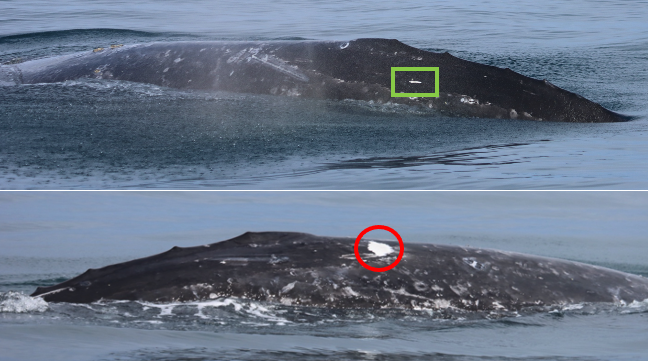
Our superstar whale Solé. Her identifying features are a small white line on her left side (green box) and a white dot in front of her dorsal hump on the right side (red circle). Source: GEMM Lab. Photograph captured under NOAA/NMFS permit #21678
Just a week after this trial day, we had our official start to the field season with back-to-back days on the water. On our first day, postdoc Alejandro, Clara and I were joined by St. Andrews University Research Fellow Enrico Pirotta, who is another member of the GRANITE team. Enrico’s role in the GRANITE project is to implement our long-term, replicate dataset into a framework called Population consequences of disturbance (PCoD; you can read all about it in a previous blog). We were thrilled that Enrico was able to join us on the water to get a sense for the species and system that he has spent the last several months trying to understand and model quantitatively from a computer halfway across the world. Luckily, the whales sure showed up for Enrico, as we saw a total of seven whales, all of which were known individuals to us! Several of the whales were feeding in water about 20 m deep and surfacing quite erratically, making it hard to get photos of them at times. Our on-board fish finder suggested that there was a mid-water column prey layer that was between 5-7 m thick. Given the flat, sandy substrate the whales were in, we predicted that these layers were composed of porcelain crab larvae. Luckily, we were able to confirm our hypothesis immediately by dropping a zooplankton net to collect a sample of many porcelain crab larvae. Porcelain crab larvae have some of the lowest caloric values of the nearshore zooplankton species that gray whales likely feed on (Hildebrand et al. 2021). Yet, the density of larvae in these thick layers probably made them a very profitable meal, which is likely the reason that we saw another five whales the next day feeding on porcelain crab larvae once again.
Porcelain crab larvae. Source: GEMM Lab.A happy captain Ale! Source: GEMM Lab.Enrico (right) and myself after collecting a large fecal sample. Source: GEMM Lab.
On our most recent field work day, we only encountered Solé, suggesting that the porcelain crab swarms had dissipated (or had been excessively munched on by gray whales), and many whales went in search for food elsewhere. We have done a number of zooplankton net tows across our study area and while we did collect a good amount of mysid shrimp already, they were all relatively small. My prediction is that once these mysids grow to a more profitable size in a few days or weeks, we will start seeing more whales again.
The GRANITE team from above, waiting & watching for whales, as we will be doing for the rest of the summer! Source: GEMM Lab.
So far we have seen nine unique individuals, flown the drone over eight of them, collected fecal samples from five individuals, conducted 10 zooplankton net tows and seven GoPro drops in just four days of field work! We are certainly off to a strong start and we are excited to continue collecting rock solid GRANITE data this summer to continue our efforts to understand gray whale ecology and physiology.
Literature cited
Hildebrand L, Bernard KS, Torres LGT. 2021. Do gray whales count calories? Comparing energetic values of gray whale prey across two different feeding grounds in the Eastern North Pacific. Frontiers in Marine Science 8. doi: 10.3389/fmars.2021.683634
Over six field seasons the GEMM lab team has conducted nearly 500 drone flights over gray whales, equaling over 100 hours of footage. These hours of footage are the central dataset for my PhD dissertation, so it’s up to me to process them all. This process can be challenging, tedious, and daunting, but it is also quite fun and a privilege to be the one person who gets to watch all the footage. It’s fascinating to get to know the whales and their behaviors and pick up on patterns. It motivates me to get through this video processing step and start doing the data analysis. Recently, it’s been especially fun to notice patterns that I’ve seen mentioned in the literature. One example is adult social behavior.
There are two categories of social behavior that I’m interested in studying: maternal behavior, defined as interactions between a mom and its calf, and general social behaviors, defined as social interactions between non-mom/calf pairs. In this blog I’ll focus on general social behaviors, but if you’re interested in maternal behavior check out this blog. General social behavior, which I’ll refer to as social behavior moving forward, includes tactile interactions and promiscuous behaviors (Torres et al. 2018; Clip 1). While gray whales in the PCFG range are primarily foraging, researchers have observed increases in social behavior towards the end of the foraging season (Stelle et al., 2008; Torres et al., 2018). We think that this indicates that the whales are starting to focus less on feeding and more on breeding. This tradeoff of foraging vs. socializing time is interesting because it comes at an energetic cost.
Clip 1. Example of social interaction between a male and female gray whale off the coast of Oregon, USA. Collected under NOAA/NMFS permit #21678
Broadly, animals need to balance the energetic demands of survival with those of reproduction. They need to reproduce to pass on their genes, but reproduction is energetically demanding, and animals also need to survive and grow to be able to reproduce. The decision to reproduce is costly because reproduction requires energetic investment and time investment since animals do not forage (gaining energy) when they are socializing. Consequently, only animals with sufficient energy reserves (i.e., body condition) to invest in reproduction actually engage in reproduction. Given these costs associated with reproduction, we expect to see a relationship between social behavior and body condition (Green, 2001) with mainly animals in good body condition engaging in social behavior because these animals have sufficient reserves to sustain the cost. Furthermore, since body condition is an indicator of foraging success and prey availability, environmental conditions can also affect social behavior and reproduction through this pathway.
Rahman et al. (2014) used a lab experiment to study the relationship between nutritional stress and male guppy courtship behavior (Figure 1). In their experiment they tested for the effects of both decreased diet quantity and quality on the frequency of male courtship behaviors. Rahman et al (2014) found that individuals in the low-quantity group were significantly smaller than those in the high-quality group and that diet quantity had a significant effect on the frequency of courtship behaviors. Males fed a low-quantity diet performed fewer courtship behaviors. Interestingly, there was no significant effect of diet quality on courtships behavior, although there was some evidence of an interaction effect, which suggests that within the low-quantity group, males fed with high-quality food performed more courtship behaviors that those fed with low-quality food. This study is interesting because it shows how foraging success (diet quantity and quality) can affect courting behavior.
Figure 1. A guppy (Rahman et al., 2013)
However, guppies are not the ideal species for comparison to gray whales because gray whales and guppies have quite different life history traits. A more fitting comparison would be with an example species with more in common with gray whales, such as viviparous capital breeders. Viviparous animals develop the embryo inside the body and give live birth. Capital breeders forage to build energy reserves and then rely on those energy reserves during reproduction. Surprisingly, I found asp vipers to be a good example species for comparison to gray whales.
Asp vipers (Figure 2) are viviparous snakes who are considered capital breeders because they forage prior to hibernation, and then begin reproduction immediately following hibernation without additional foraging. Naulleau & Bonnet (1996) conducted a field study on female asp vipers to determine if there was a difference in body condition at the start of the breeding season between females who reproduced or not during that season. To do this they marked individuals and measured their body condition at the start of the breeding season and then recaptured those individuals at the end of the breeding season and recorded whether the individual had reproduced. Interestingly, they found that there was a strongly significant difference in body condition between females that did and did not reproduce. In fact, they discovered that no female below a certain body condition value reproduced, meaning that they found a body condition threshold for reproduction.
Figure 2. An asp viper
Additionally, a study on water pythons found that their body condition threshold for reproduction shifted over time in response to prey availability (Madsen & Shine, 1999). These authors found that females lowered their threshold after several consecutive years of poor prey availability. These studies are really exciting to me because they address questions that the GRANITE project team is interested in tackling.
Understanding the relationship between body condition and reproduction in gray whales is an important puzzle piece for our work. The aim of the GRANITE project is to understand how the effects of stressors on individual whales scales up to population level impacts (read Lisa’s blog to learn more). Reproduction rates play a big role in population dynamics, so it is important to understand what factors affect reproduction. Since we’re studying these whales on their foraging grounds, assessing body condition provides an important link between foraging behavior and reproduction.
For example, if an individual’s response to a stressor is to forage less, that may lead to poorer body condition, meaning that they may be less likely to reproduce. While reduced reproduction in one individual may not have a big effect on the population, the same response from multiple individuals could impact the population’s dynamics (i.e., increasing or decreasing abundance). Understanding these different relationships between behavior, body condition, and reproduction rates is a big undertaking, but it’s exciting to be a member of the GRANITE team as this strong group of scientists works to bring together different data streams to work on this big picture question. We’re all deep into data processing right now so stay tuned over the next few years to learn more about gray whale social behavior and to find out if fat whales are more social than skinny whales.
Did you enjoy this blog? Want to learn more about marine life, research, and conservation? Subscribe to our blog and get weekly updates and more! Just add your name into the subscribe box on the left panel.
References
Green, A. J. (2001). Mass/Length Residuals: Measures of Body Condition or Generators of Spurious Results? Ecology, 82(5), 1473–1483. https://doi.org/10.1890/0012-9658(2001)082[1473:MLRMOB]2.0.CO;2
Madsen, T., & Shine, R. (1999). The adjustment of reproductive threshold to prey abundance in a capital breeder. Journal of Animal Ecology, 68(3), 571–580. https://doi.org/10.1046/j.1365-2656.1999.00306.x
Naulleau, G., & Bonnet, X. (1996). Body Condition Threshold for Breeding in a Viviparous Snake. Oecologia, 107(3), 301–306.
Rahman, M. M., Kelley, J. L., & Evans, J. P. (2013). Condition-dependent expression of pre- and postcopulatory sexual traits in guppies. Ecology and Evolution, 3(7), 2197–2213. https://doi.org/10.1002/ece3.632
Rahman, M. M., Turchini, G. M., Gasparini, C., Norambuena, F., & Evans, J. P. (2014). The Expression of Pre- and Postcopulatory Sexually Selected Traits Reflects Levels of Dietary Stress in Guppies. PLOS ONE, 9(8), e105856. https://doi.org/10.1371/journal.pone.0105856
Stelle, L. L., Megill, W. M., & Kinzel, M. R. (2008). Activity budget and diving behavior of gray whales (Eschrichtius robustus) in feeding grounds off coastal British Columbia. Marine Mammal Science, 24(3), 462–478. https://doi.org/10.1111/j.1748-7692.2008.00205.x
Torres, L. G., Nieukirk, S. L., Lemos, L., & Chandler, T. E. (2018). Drone up! Quantifying whale behavior from a new perspective improves observational capacity. Frontiers in Marine Science, 5(SEP). https://doi.org/10.3389/fmars.2018.00319
Clara Bird, PhD Student, OSU Department of Fisheries, Wildlife, and Conservation Sciences, Geospatial Ecology of Marine Megafauna Lab
When I thought about what doing fieldwork would be like, before having done it myself, I imagined that it would be a challenging, but rewarding and fun experience (which it is). However, I underestimated both ends of the spectrum. I simultaneously did not expect just how hard it would be and could not imagine the thrill of working so close to whales in a beautiful place. One part that I really did not consider was the pre-season phase. Before we actually get out on the boats, we spend months preparing for the work. This prep work involves buying gear, revising and developing protocols, hiring new people, equipment maintenance and testing, and training new skills. Regardless of how many successful seasons came before a project, there are always new tasks and challenges in the preparation phase.
For example, as the GEMM Lab GRANITE project team geared up for its seventh field season, we had a few new components to prepare for. Just to remind you, the GRANITE (Gray whale Response to Ambient Noise Informed by Technology and Ecology) project’s field season typically takes place from June to mid-October of each year. Throughout this time period the field team goes out on a small RHIB (rigid hull inflatable boat), whenever the weather is good enough, to collect photo-ID data, fecal samples, and drone imagery of the Pacific Coast Feeding Group (PCFG) gray whales foraging near Newport, OR, USA. We use the data to assess the health, ecology and population dynamics of these whales, with our ultimate goal being to understand the effect of ambient noise on the population. As previous blogs have described, a typical field day involves long hours on the water looking for whales and collecting data. This year, one of our exciting new updates is that we are going out on two boats for the first part of the field season and starting our season 10 days early (our first day was May 20th). These updates are happening because a National Science Foundation funded seismic survey is being conducted within our study area starting in June. The aim of this survey is to assess geophysical structures but provides us with an opportunity to assess the effect of seismic noise on our study group by collecting data before, during, and after the survey. So, we started our season early in order to capture the “before seismic survey” data and we are using a two-boat approach to maximize our data collection ability.
While this is a cool opportunistic project, implementing the two-boat approach came with a new set of challenges. We had to find a second boat to use, buy a new set of gear for the second boat, figure out the best way to set up our gear on a boat we had not used before, and update our data processing protocols to include data collected from two boats on the same day. Using two boats also means that everyone on the core field team works every day. This core team includes Leigh (lab director/fearless leader), Todd (research assistant), Lisa (PhD student), Ale (new post-doc), and me (Clara, PhD student). Leigh and Todd are our experts in boat driving and working with whales, Todd is our experienced drone pilot, I am our newly certified drone pilot, and Lisa, Ale, and myself are boat drivers. Something I am particularly excited about this season is that Lisa, Ale, and I all have at least one field season under our belts, which means that we get to become more involved in the process. We are learning how to trailer and drive the boats, fly the drones, and handling more of the post-field work data processing. We are becoming more involved in every step of a field day from start to finish, and while it means taking on more responsibility, it feels really exciting. Throughout most of graduate school, we grow as researchers as we develop our analytical and writing skills. But it’s just as valuable to build our skillset for field work. The ocean conditions were not ideal on the first day of the field season, so we spent our first day practicing our field skills.
For our “dry run” of a field day, we went through the process of a typical day, which mostly involved a lot of learning from Leigh and Todd. Lisa practiced her trailering and launching of the boat (figure 1), Ale and Lisa practiced driving the boat, and I practiced flying the drone (figure 2). Even though we never left the bay or saw any whales, I thoroughly enjoyed our dry run. It was useful to run through our routine, without rushing, to get all the kinks out, and it also felt wonderful to be learning in a supportive environment. Practicing new skills is stressful to say the least, especially when there is expensive equipment involved, and no one wants to mess up when they’re being watched. But our group was full of support and appreciation for the challenges of learning. We cheered for successful boat launchings and dockings, and drone landings. I left that day feeling good about practicing and improving my drone piloting skills, full of gratitude for our team and excited for the season ahead.
Figure 1. Lisa (driving the truck) launching the boat.
Figure 2. Clara (seated, wearing a black jacket) landing the drone in Ale’s hands.
All the diligent prep work paid off on Saturday with a great first day (figure 3). We conducted five GoPro drops (figure 4), collected seven fecal samples from four different whales (figure 5), and flew four drone flights over three individuals including our star from last season, Sole. Combined, we collected two trifectas (photo-ID images, fecal samples, and drone footage)! Our goal is to get as many trifectas as possible because we use them to study the relationship between the drone data (body condition and behavior) and the fecal sample data (hormones). We were all exhausted after 10 hours on the water, but we were all very excited to kick-start our field season with a great day.
Figure 3. Lisa on the bow pulpit during our first sighting of the day.
Figure 4. Lisa doing a GoPro drop, she’s lowering the GoPro into the water using the line in her hands.
Figure 5. Clara and Ale collecting a fecal sample.
On Sunday, just one boat went out to collect more data from Sole after a rainy morning and I successfully flew over her from launching to landing! We have a long season ahead, but I am excited to learn and see what data we collect. Stay tuned for more updates from team GRANITE as our season progresses!
Fall has arrived in the Pacific Northwest. For humans, it means packing away the shorts and sandals, and getting the boots, raincoats and firewood ready. For gray whales, it means gulping down the last meal of zooplankton they will eat for several months and commencing the journey to warmer waters and sunnier skies in Mexico where they will spend the winter fasting, calving, and nursing. While the GEMM Lab may still squeeze in a day or two of field work this week, we are slowly wrapping up the 2020 field season as conditions get rougher and our beloved gray whales gradually depart our waters. This year marked the 6th year of data collection for both of our gray whale projects: the Newport project that investigates the impacts of multiple stressors on gray whale ecology and health, and the Port Orford project that explores fine-scale foraging ecology of gray whales and their zooplankton prey. Since it will be several months before the GEMM Lab heads back out onto the water again, I thought I would summarize our two field seasons, share some highlights, and muse about the drivers of our observations this summer.
Some snapshots of the field team hard at work this summer. Top left: Hunter Warwick operating the drone. Top right: PI Leigh Torres rocking the lab swag to protect against the sun. Bottom left: Lisa Hildebrand waiting for a whale to surface to get photos of it. Bottom right: Alejandro Fernandez Ajo transfers zooplankton from the light trap to sample jars.
Summaries
Our RHIB Ruby zipped around the central and southern Oregon coast on 33 different days. The summer started slow, with several days of field work where we encountered no whales despite surveying our entire study region. Our encounters picked up towards the end of June and by the end of the summer we totaled 107 sightings, encountering 46 unique individuals, 36 of which were resightings of known individuals we have identified in previous years. Our Newport star of the summer was Solé, a female gray whale we have seen every year since 2015, and we also saw many of our other regulars including Casper, Rafael, Spray, Bit, and Heart. None of these whales shone as bright as Solé though. We flew the drone over her 8 times and collected 7 fecal samples (one of which was the biggest whale fecal sample I have ever seen!). In total, we collected 30 fecal samples and flew the drone 88 times. These data will allow us to continue measuring body condition and hormone levels of Pacific Coast Feeding Group (PCFG) gray whales that use the Oregon coast.
Left: Our RHIB Ruby heading out for a day of field work in Port Orford, OR this summer. Right: Solé. Image captured under NOAA/NMFS permit #21678.
Our tandem research kayak Robustus may not be as zippy as Ruby (it is powered by human muscle rather than a powerful outboard engine after all), but it certainly continues to be a trusty vessel for the Port Orford team. The Port Orford research team, named the Theyodelers this year, collected 181 zooplankton samples and conducted 180 GoPro drops during the month of August from Robustus. Despite the many samples collected, the size of our prey samples remained relatively small throughout the whole season compared to previous years. The cliff team surveyed for a total of 117 hours, of which 15 were spent tracking whales with the theodolite and resulted in 40 different tracklines of whale movements. The whale situation in Port Orford was similar to the pattern of whale sightings in Newport, with low whale sightings at the start of the field season. Luckily, by the start of August (which marked the start of data collection for the Theyodelers), the number of whales using the Port Orford area, especially the two study sites, Mill Rocks & Tichenor Cove, had increased. Of the whales that came close enough to shore for us to identify using photo-id, we tracked 5 unique individuals, 3 of which we also saw in Newport this year. The Port Orford star of the summer was Smudge, with his tracklines making up a quarter of all of our tracklines collected. Smudge is also the whale we sighted most often last year in Port Orford.
Top: Theyodelers Mattea Holt Colberg and Liz Kelly sampling atop the kayak Robustus. Bottom: Smudge. Image captured under NOAA/NMFS permit #21678.
Highlights
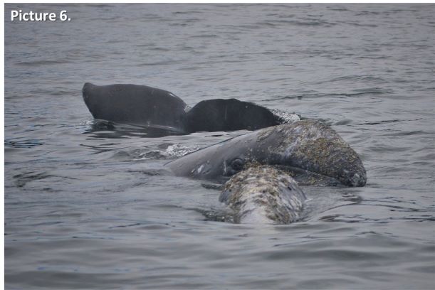
Many of you may be familiar with the whale Scarlett (formally known as Scarback). Scarlett is a female, at least 24 years old (she was first documented in the PCFG range in 1996), who is well-known (and easily identified) by the large concave injury on her back that is covered in whale lice, or cyamids. No one knows for certain how Scarlett sustained this injury (though there are stories), however what we do know is that it has not prevented this female from reproducing and successfully raising several calves over her lifetime. The GEMM Lab last saw Scarlett with a calf (which we named Brown) in 2016. Since Scarlett is such a famous whale with a unique history, it shouldn’t be a surprise that one of our highlights this summer is the fact that Scarlett showed up with a new calf! In keeping with a “shades of red” theme, Leigh came up with the name Rose for the new calf. In July, the mom-calf pair put on quite a cute performance, with Rose rising up on Scarlett’s back, giving the team a glimpse of its face. The Scarlett-Rose highlight doesn’t end there though. Just last week, we had a very brief encounter in choppy, swelly waters with a small whale. The whale surfaced just twice allowing us to capture photo-id images, and as we were looking around to see where it would come up a third time, it suddenly breached approximately 20 m from the boat. Lo-and-behold, after comparing our photos of the whale to our catalogue, we realized that this elusive, breaching whale was Rose! I am excited to see whether Rose will return to the Oregon coast next summer and become a PCFG regular just like her mom.
Top: Scarlett, easily identified by the large concave injury on her back covered in cyamids. Bottom: Scarlett with her new calf Rose riding her back, giving us a glimpse of its face. Images captures under NOAA/NMFS permit #21678.
The highlight of the field season in Port Orford is the trial, failures and small successes of a new element to the project. There is still a lot that we do not know and understand about PCFG gray whales. One such thing is the way in which gray whales maneuver their large bodies in shallow rocky habitats, often riddled with kelp, and how exactly they capture their zooplankton prey in these environments. Using drones has certainly helped bring some light into this darkness and has led to the documentation of many novel foraging behaviors (Torres et al. 2018). However, the view from above is unable to provide the fine-scale interactions between whales, kelp, reefs, and zooplankton. Instead, we must somehow find a way to watch the whales underwater. Enter CamDo. CamDo is a technology company that designs specialty products to allow for GoPro cameras to be used for time-lapsed recordings over long periods of time in harsh environmental conditions. One of their products is a housing specifically designed for long-term filming underwater – exactly what we need! The journey was not as easy as simply purchasing the housing. We also needed to build a lander for the housing to sit on (thankfully our very own Todd Chandler designed and built something for us), and coordinate with divers and a vessel to deploy and retrieve the set-up, as well as undertake weekly battery and SD cards swaps (thankfully Dave Lacey of South Coast Tours and a very generous group of divers* donated their time and resources to make this happen). We unfortunately had some technological difficulties and bad visibility for the first 4 weeks (precisely why this CamDo effort was a pilot season this year), however we had some small success in the last 2 weeks of deployment that give us hope for the future. The camera recorded a lot of things: thick layers of mysids, countless rockfish and lingcod, several swimming and foraging murres, a handful of harbor seals, and two encounters of the species we were hoping to film – gray whales! While the footage is not the ‘money shot’ we are hoping to film (aka, a headstanding gray whale eating zooplankton right in front of the camera), the fact that we captured gray whales in the first place has showed us that this set-up is a promising investment of time, money and effort that will hopefully deliver next year.
Top left: CamDo atop its lander designed and built by Todd Chandler. Top right: Divers getting ready to get into the water for a battery and SD card swap. Bottom: Dave Lacey and two of our divers with the Black Pearl, South Coast Tour’s boat.
Musings
You may have picked up on the fact that we had slow starts to our field seasons in both Newport and Port Orford. Furthermore, while the number of whale sightings did increase in both locations throughout the field seasons, the number of sightings and whales per day were lower than they have been in previous years. For example, in 2018, we identified 15 different individuals in the month of August in Port Orford (compared to just 5 this year). In 2019, 63 unique whales were seen in Newport (compared to 46 this year). Interestingly, we had a greater diversity of encountered individuals at the start and end of the season in Newport, with a relatively small number of different individuals in July and August. While I cannot provide a definitive reason (or reasons) as to why patterns were observed (we will need to analyze several years of our data to try and understand why), I have some hypotheses I wish to share with you.
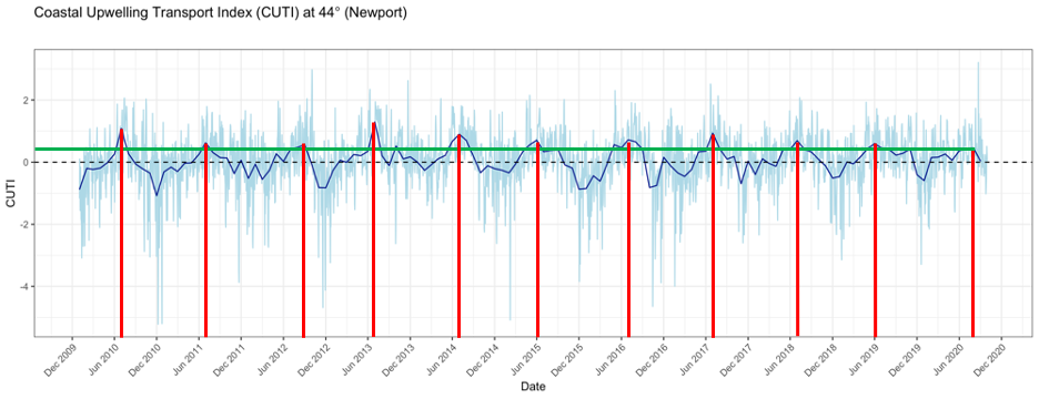
As I mentioned in a previous blog, this summer the coastal upwelling along the Oregon coast was delayed (Figure 1). Typically, peak upwelling occurs during the month of June or shortly thereafter, bringing nutrient-rich, deep waters to the surface and, when mixed with sunlight, a lot of productivity. This productivity sets off a chain of reactions — the input of nutrients leads to increased phytoplankton production, which in turn leads to increased zooplankton production, resulting in growth and development of larger organisms that consume zooplankton, such as rockfish and gray whales. If the timing of upwelling is delayed, then so too is this chain of reactions. As you can see from Figure 1, the red lines show that the peak upwelling this year occurred far later in the summer than any year in the last 10 years, with the exception of 2012. Gray whales may have cued into this delay and therefore also delayed their arrival to the PCFG feeding grounds, hence causing us to have low sighting rates at the start of our season. However, this is mostly speculative as we still do not understand the functional mechanisms by which cetaceans, such as gray whales, detect prey across different scales, and to what extent oceanographic conditions like upwelling may play a role in prey availability (Torres 2017).
Figure 1. 10 year time series of the Coastal Upwelling Transport Index (CUTI). CUTI represents the amount of upwelling (positive numbers) or downwelling (negative numbers). The light-colored lines representthe CUTI at that point in time while the dark, bold line represents the long-term average.The vertical red lines represent the point of peak upwelling in that summer and the horizontal green line shows the peak level of upwelling in 2020 relative to all previous years.
Furthermore, the green line in Figure 1shows that even after peak upwelling was reached this year, upwelling conditions were lower than all the other peaks in the previous 10 years. We know that weak upwelling is correlated to poor body condition of PCFG gray whales in subsequent years (Soledade Lemos et al. 2020). Upon arriving to the Oregon coast feeding grounds, gray whales may have noticed that it was shaping up to be a poor prey year (we certainly noticed it in Port Orford in the emptiness of our zooplankton net). Faced with this low resource availability, individuals had to make important decisions – risk staying in a currently prey-poor environment or continue the journey onward, searching for better prey conditions elsewhere. This conundrum is known as the marginal value theorem, whereby an individual must decide whether it should abandon the patch it is currently foraging on and move on to search for a new patch without knowing how far away the next patch may be or its value relative to the current patch (Charnov 1976). If we think of the Oregon coast as the ‘current patch’, then we can see how the marginal value theorem translates to the situation gray whales may have found themselves in at the start of the summer.
Yet, an individual gray whale does not make these decisions in a vacuum. Instead, all gray whales in the same area are faced with the same conundrum. Seminal work by Pianka (1974) showed that when resources, such as food, are abundant, then competition between predators is low because there is enough food to go around. However, when resources dwindle, competition increases and the niches of predators begin to overlap more and more. With Charnov and Pianka’s theories in mind, we can see two groups of gray whales emerge from our 2020 field work observations: those that stayed in the ‘current patch’ (Oregon) and those that decided to seek out a new patch in hopes that it would be a better one. Solé certainly belongs in the first group. We saw her consistently throughout the whole summer. In fact, she was oftentimes so predictable that we would find her foraging on the same reef complex every time we went out to survey. Smudge may also belong in this group, however it is hard to say definitively since we only survey in Port Orford in late July and August. In contrast, I would place whales such as Spray and Heart in the second group since we saw them early in the summer and then not again until mid-to-late September. Where did they go in the interim? Did they go somewhere else in the PCFG range? Or did they venture all the way up to Alaska to the primary Eastern North Pacific (ENP) gray whale feeding grounds? Did their choice to search for food elsewhere pay off?
As I said earlier, these are all just musings for now, but the GEMM Lab is already hard at work trying to answer these questions. Stay tuned to see what we find!
* Thanks to all the divers who assisted with the pilot CamDo season: Aaron Galloway, Ross Whippo, Svetlana Maslakova, Taylor Eaton, Cori Kane, Austin Williams, Justin Smith
References
Charnov, E.L. 1976. Optimal Foraging, the Marginal Value Theorem. Theoretical Population Biology 9(2):129-136.
Pianka, E.R. 1974. Niche Overlap and Diffuse Competition. PNAS 71(5):2141-2145.
Soledade Lemos, L., Burnett, J.D., Chandler, T.E., Sumich, J.L., and L.G. Torres. 2020. Intra- and inter-annual variation in gray whale body condition on a foraging ground. Ecosphere 11(4):e03094.
Torres, L.G. 2017. A sense of scale: Foraging cetaceans’ use of scale-dependent multimodal sensory systems. Marine Mammal Science 33(4):1170-1193.
Torres, L.G., Nieukirk, S.L., Lemos, L., and T.E. Chandler. 2018. Drone Up! Quantifying Whale Behavior From a New Perspective Improves Observational Capacity. Frontiers in Marine Science: https://doi.org/10.3389/fmars.2018.00319.
By Alejandro Fernandez Ajo, PhD student at the Department of Biology, Northern Arizona University, Visiting scientist in the GEMM Lab working on the gray whale physiology and ecology project
Two years ago, in August 2018, I came to Newport and visited the Hatfield Marine Science Center for the first time with an NSF/RCN-founded laboratory exchange with the GEMM Lab and met Dr. Leigh Torres. My goals during this exchange where to learn about non-invasive fieldwork techniques for studying free-range whales while interacting, exchanging ideas, and networking with the GEMM Lab members; also, to discuss some projects and thoughts for future collaborations with Dr. Torres. During those two weeks in Newport, I had the opportunity to help with field work on the project “Evaluation of gray whale ecology and physiology in response to variable ambient ocean noise conditions”, which aims to evaluate the hormonal variability and health of the gray whales that forage along the Oregon coast in the context of multiple stressors. I would return during the summers of 2019 and 2020 as a visiting scientist and research assistant to work on this project. This year the experience has been a bit different in terms of interactions with the HMSC community due to COVID-19; however, we were able to successfully start the field season in time and now we are wrapping up our second month of surveys with many new and interesting data gathered, and many new, unforgettable memories to be treasured. Working with these animals is incredibly fascinating because there are so many things we don´t know about them, and the questions can become both overwhelming and exciting.
An essential part of this project, and arguably any research project done with cetaceans, is the identification of individuals. Hence, considerable effort is expended each year attempting to photograph every gray whale possible within our study region and to identify each whale we encounter. The GEMM Lab maintains a catalog of the gray whales that visit the Oregon coast, a sub-population known as the Pacific Coast Feeding Group (PCFG). This catalog currently consists of 173 individuals. which we frequently compare with a larger catalog of gray whales that includes 2060 individuals observed since 1977 (Cascadia Research Collective). These methods allow us to know who is who among the whales we encounter each day at sea.
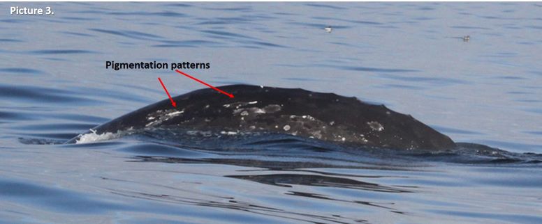
The different species of cetaceans can be individually identified by markings on their bodies, very much like fingerprints in humans. Some features on these animals are unique and conserved through life. For example, Southern and Northern right whales are identified by the callosity patters in their heads (Picture 1), while humpback whales are mostly identified individually by the shape and the patterns of black and white pigmentation on the underside of their fluke (Picture 2). Gray whales have very mottled skin coloration, so we use a combination of markings and features to identify individuals: pigmentation patterns, scars, shape and pigmentation of their fluke, and sometimes the shape of their knuckles, which are a series of “humps” that gray whales have instead of a dorsal fin on their back. It might sound very difficult to do, and it can be a tedious task, however as you train your eye it becomes easier, and features that at first seemed undistinguishable become recognizable and unique (Picture 3). As a reward, it is such a joy to find a match and recognize old friends when they arrive from their long journeys in the vast ocean each year to the Oregon coast.
The callosity pattern of a southern right whale.Photo by Alejandro Fernández Ajó – Instituto de Conservación de Ballenas.Three different humpback whales with notably different pigmentation patterns on their flukes. Photographs captured under NOAA/NMFS permit #21678.The gray whale “Knife” we have observed frequently this summer off the Oregon coast. Can you see how the right pigmentation pattern identified looks like a knife? Photograph captured under NOAA/NMFS permit #21678.
As a result of our photo-identification efforts and the high site-fidelity of the whales we study, the large majority of the gray whales we observe here in Oregon are known individually. For many whales, we also have detailed sightings records that can span years and decades, that document calving history, lactation, appearance of scars indicative of injury or entanglement, minimum age, sex, habitat-use patterns, behaviors, etc. Holding such detailed information of individual whales provides incredible contributions to our understanding of the basic patterns in life history of whales, such as reproduction rates, calving intervals, age of first reproduction, etc. Moreover, when these life history events are linked with physiological sample collection large steps can be made in the development and validation of physiological methods. Many endocrine assays currently in use for whales are based on non-traditional sample types including feces, respiratory vapor, and baleen, which have been validated using the catalogs of well-known individuals to verify that measured hormones reflect patterns expected for various physiological states. For example, we can compare endocrine data of confirmed pregnant females, known mature males, and known-injured whales to learn how whale physiological responses are different during different life history events (e.g., Burgess et al. 2017, 2018, Corkeron et al. 2017, Hunt et al. 2006, 2016, 2018, Lysiak et al. 2018, Rolland et al. 2005).
Here in Oregon we are learning from the lives of the gray whales we study, and here I want to share with you two of their stories, one happy and one not-so-happy.
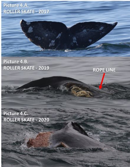
Let´s start with the not-so-happy story so we can end with some brighter news. On June 24 this year, we encountered a whale near Cape Foulweather, which is a very tricky area to work as there are many rocks and shallow water that make the sea conditions very choppy even with low swell. We started documenting the sighting as usual, taking pictures of the left side, the right side and ideally also the fluke of the whale. As we approached this whale, we started noting that something was wrong with its fluke. With the challenging sea conditions, it was not easy to approach the whale and the whale was not exposing its fluke when diving. When we put our drone up to collect photogrammetry and behavior data we gained a much better perspective. This whale has a bad injury on it fluke (Picture 4.C). On the boat we started making conjectures about the cause of this terrible injury that had basically amputate most of its left fluke lobe. Once back on shore, we sorted out the photos and compared the field images captured during the day with the photo-ID catalog and we made a match. This whale is known in our catalog as “ROLLER SKATE”, is a female, and was first sighted in 2015, so she is at least 5 years old today.
The story unfolded when we reviewed Roller Skate’s sighting history. Interestingly we observed this same whale in the same location last September 2019. Unfortunately, it was a very brief encounter but enough for photo documentation of the whale and an interesting observation. Here I quote the field notes that Dr. Torres wrote from this sighting: “September 6th, 2019. Sighting 9: Scattered whales feeding and/or traveling across area to north of Cape Foulweather. One whale had recently chopped fluke; tried to re-find to get better photos but could not (looking at photos now, this whale is clearly entangled in line!). Ceiling too low for UAS [drone flight].” (Picture 4.B).
Progressive photos of Roller Skate’s fluke. In 2017, her fluke was healthy (A). In 2019, we observed her fluke with a line entanglement and “chewed up” (B). In 2020, we have observed the resulting wound and healing process (C). Photographs captured under NOAA/NMFS permit #21678.
Roller skate’s story is an example of how essential is to keep an ID catalog. After a close-up examination of the 2019 picture, we can clearly see a rope entanglement (Picture 4.B). Photos from previous years show how beautiful and healthy her fluke was before this event (Picture 4.A). This event is heart breaking to witness, but this whale could be considered lucky because she was able to shed the gear and survive this entanglement, at least in the short term. Additionally, we can learn from Roller Skate’s misfortune to help us understand what the consequences of such an injury (stressor) may be on the physiology of a whale. We have been eager to collect a fecal sample from Roller Skate to analyze how her hormone levels compare to non-injured whales. Fortunately, we got lucky a couple weeks ago and collected this sample, so now we need to get in the lab and analyze the samples. But more questions remain: Will this injury impact her ability to reproduce? If so, for how long? And at a larger scale, what are the population consequences of such events? If we can understand the magnitude of lethal and sublethal human caused impacts on individual whales and their populations from events such as entanglements, we can develop better methods to mitigate and limit such hazards for whales in their environments.
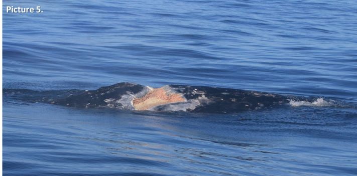
As I promised, there is also some good news to share. A very well-known PCFG whale, almost a celebrity I dear to say, is “Scarback”, or as we like to call her “Scarlett”. Scarlett is a female known since 1996, making her at least 24 years old, and she also has a very bad injury of unknown origin. Scarlett has a terrible scar on her back that is theorized to have been caused by an explosive harpoon, or maybe a bad ship-strike (Picture 5), but we really do not know. However, we do know she survived this injury and this year she brought a new calf into the population (Picture 6). This is the second calf we have documented from Scarlett, with her previous calf sighted during the 2016 field season and we call it “Brown”. Scarlett is an example of how resilient these amazing giants can be; however, it is likely that while she was recovering from this injury, she was unable to reproduce. How many calves from Scarlett did the PCFG population “lose” due to such a tragedy? We can´t know, but we are learning, and her story will also help us understand whale physiology as we will analyze her fecal hormones and body condition during pregnancy, lactation, and resting phases.
The scar on Scarlett’s back. This significant wound has an unknown origin.Photograph captured under NOAA/NMFS permit #21678.
Scarlett is a survivor. We need to recognize that we are sharing the ocean with different forms of life. We need to acknowledge their existence and understand how our use of the oceans is affecting them, and, more importantly, work toward improving their conditions. I hope that with our research we highlight and communicate how amazing are these animals, and how important are they for marine ecosystems. And ultimately, I hope our work helps minimize the impacts that affect other forms of ocean life that coexist with us, both above and below the surface.
The well-known gray whale “Scarlett” surfaces under her calf while it checks out the GEMM Lab field team. Photo by Alejandro Fernandez Ajo taken under NOAA/NMFS permit #21678.
References:
Burgess, E., Hunt, K. E., Kraus, S. D. and Rolland, R. M. (2016). Get the most out of blow hormones: validation of sampling materials, field storage and extraction techniques for whale respiratory vapor samples. Conservation Physiology, 4, cow024.
Burgess, E. A., Hunt, K. E., Kraus, S. D. and Rolland, R. M. (2018). Quantifying hormones in exhaled breath for physiological assessment of large whales at sea. Scientific Reports, 8, 10031.
Corkeron, P. J., Rolland, R. M., Hunt, K. E. and Kraus, S. D. (2017). A right whale PooTree: Fecal hormones and classification trees identify reproductive states in North Atlantic right whales (Eubalaena glacialis). Conservation Physiology, 5, cox006. DOI: 10.1093/conphys/cox006.
Hunt, K., Lysiak, N., Moore, M. and Rolland, R. (2017). Multi-year longitudinal profiles of cortisol and corticosterone recovered from baleen of North Atlantic right whales (Eubalaena glacialis). General and Comparative Endocrinology, 254, 50-59. DOI: 10.1016/j.ygcen.2017.09.009.
Hunt, K., Lysiak, N. S. J., Matthews, C. J. D., et al. (2018). Multi-year patterns in testosterone, cortisol and corticosterone in baleen from adult males of three whale species. Conservation Physiology, 6, coy049. DOI: 10.1093/conphys/coy049.
Hunt, K. E., Rolland, R. M., Kraus, S. D. and Wasser, S. K. (2006). Analysis of fecal glucocorticoids in the North Atlantic Right Whale (Eubalaena glacialis). General and Comparative Endocrinology, 148, 260-272.
Lysiak, N., Trumble, S., Knowlton, A. and Moore, M. (2018). Characterizing the duration and severity of fishing gear entanglement on a North Atlantic right whale (Eubalaena glacialis) using stable isotopes, steroid and thyroid hormones in baleen. Frontiers in Marine Science. DOI: 10.3389/fmars.2018.00168.
Rolland, R. M., Hunt, K. E., Kraus, S. D. and Wasser, S. K. (2005). Assessing reproductive status of right whales (Eubalaena glacialis) using fecal hormone metabolites. General and Comparative Endocrinology, 142, 308-317.
By Hunter Warick, Research Technician, Geospatial Ecology of Marine Megafauna Lab, Marine Mammal Institute
When monitoring the health of a capital breeding species, such as whales that store energy to support reproduction costs, it is important to understand what processes and factors drive the status of their body condition. Information gained will allow for better insight into their cost of reproduction and overall life history strategies.
For the past four years the GEMM Lab has utilized the perspective that Unoccupied Aerial Systems (UAS; or ‘drones’) provide for observations of marine mammals. This aerial perspective has documented gray whale behavior such as jaw snapping, drooling mud, and headstands, all of which shows or suggest foraging (Torres et al. 2018). However, UAS is limited to a bird’s eye view, allowing us to see WHAT whales are doing, but limited information about the reasons WHY. To overcome this hurdle, Leigh Torres and team have equipped their marine mammal research utility belts with the use of GoPro cameras. They developed a technique known as the “GoPro drop” where a GoPro camera mounted to a weighted pole is lowered off the side of the research vessel in waters < 20 m deep via a line to record video data. This technique allows the team to obtain fine-scale habitat and prey variation information, like what the whale experiences. Along with the context provided by the UAS, this dual camera perspective allows for deeper insight into gray whale foraging strategies and efficiency. Torres’s GoPro data analysis protocol examines kelp density, kelp health, benthic substrate, rock fish density, and mysid density. These characteristics are graded along a scale (Figure 1), allowing for relative comparisons of habitat and prey availability between where whales spend time and forage. These GoPro drops will also help create a fine-scale benthic habitat map of the Newport field area. So, why are these data on gray whale habitat and prey important to understand?
Figure 1. The top row shows varying degrees of mysid density (low to high, left to right). Middle row illustrates different types of substrate you might encounter (reef, sandy, boulders; left to right). Bottom row shows the different levels of kelp health (poor, medium, good).
The foraging grounds are the first step in the life history domino chain reaction for many rorqual whales; if this step doesn’t go off cleanly then everything else fails to fall into place. Gray whales partake on a 15,000-20,000 km (round trip) migration, which is the longest of any known mammal (Swartz 1986). During this migration, whales spend around three months fasting in their breeding grounds (Highsmith & Coyle 1992), living only off the energy stores that they accumulated in their feeding grounds (Næss et al. 1998). These extreme conditions of existence for gray whales drive the need to be a successful forager and is why it is so crucial for them to forage in high prey density areas (Newell, C. 2009).
Mysids are a critical part of the gray whale diet in Oregon waters (Newell, C. 2009; Sullivan, F. 2017) and mysids have strong predator-prey relationships with both top-down and bottom-up control (Dunham & Duffus 2001; Newell & Cowles 2006). This unique tie illustrates the great dependency that gray whales have on mysids, further showing the benefit to looking at the density of mysids where gray whales are seen foraging. The quality of mysids may also be as important as quantity; with higher water temperatures resulting in lower lipid content in mysids (Mauchline 1980), suggesting density might not be the only factor for determining efficient whale foraging. The overall goal of gray whales on their foraging grounds is to get as fat as possible in order to reproduce as often as possible. But, this isn’t always as easy as it sounds. Gray whales typically have a two-year breeding interval but can be anywhere from 1-4 years (Blokhin 1984). The longer time it takes to build up adequate energy stores to support reproduction costs, the longer it will take to breed successfully. Building back up these energy stores can prove to be difficult, especially for lactating females (Figure 2).
Figure 2. Comparison of body condition between a lactating female gray whale on the feeding grounds in Newport, Oregon, 2020 (GEMM Lab, OSU; NOAA/NMFS permit # 21678) and a pregnant female gray whale on the breeding grounds in San Ignacio Lagoon, 2019 (provided by Laguna San Ignacio Ecosystem Program). Photographer Hunter Warick. Note the very different body shapes: thin lactating female relative to the rotund pregnant female.
Being able to track the health and behavior of gray whales on an individual level, including comparisons between variation in body condition, foraging behavior, and fine scale information on benthic communities gained through the use of GoPros, can provide a better understanding of the driving factors and impacts on their health and population trends (Figure 3).
Figure 3. A compilation of video clips captured by the GEMM Lab during their research on gray whale ecology and physiology off Newport, Oregon using Unoccupied Aerial Systems (UAS, or “drones”) and GoPro cameras. UAS are used to observe gray whale behavior and conduct photogrammetry assessment of body condition. GoPro camera drops assess the benthic habitat and prey density across the study region, with a couple chance encounters of whales. Research is conducted under NOAA/NMFS permit # 21678.
Every two years, an international community of scientists, managers, policy-makers, educators, and students gather to share the most current research and most pressing conservation issues facing marine mammals. This year, the World Marine Mammal Conference will take place in Barcelona, Spain from December 7-12, and the whole GEMM Lab will make their way across the Atlantic to present their latest work. The meeting is an international gathering of scientists ranging from longtime researchers who have shaped the field throughout the course of their careers to students who are just beginning to carve out a niche of their own. This year’s conference has 2,500 registered attendees from 95 different countries, 1,960 abstract submissions, and 700 accepted oral and speed talks and 1,200 posters. Needless to say, it is an incredible platform for learning, networking, and putting our work in the context of research taking place around the globe.
This will be
my third time at this conference. I attended in San Francisco in 2015 as a
wide-eyed undergraduate and met with Leigh, who I hoped would soon become my
graduate advisor. I also presented my Masters research at the conference in
Halifax in 2017. This time around, I will be presenting findings from the first
two chapters of my PhD. Looking ahead to the Barcelona 2019 meeting and having
some sense of what to expect, I feel butterflies rising in my stomach—a perfect
mixture of the nerves that come with putting your hard work out in the world,
eagerness to learn and absorb new information, and excitement to reconnect with
friends and colleagues from around the world. In short, I can’t wait!
For those of
you reading this blog that are unable to attend, I’d like to share an overview of
what the GEMM Lab will be presenting at the conference. If you will be in
Barcelona, we warmly invite you to the following posters, speed talks, and oral
presentations! In order of appearance:
Lisa Hildebrand, MS Student
What do Oregon gray whales like to eat? Do individual whales have individual foraging habits? To learn more visit Lisa Hildebrand’s poster “Investigating potential gray whale individual foraging specializations within the Pacific Coast Feeding Group”. (Poster presentation,Session: Foraging Ecology – Group A, Time: Monday, 1:30-3:00pm)
Todd Chandler, Faculty Research Assistant
Did you know it is possible to measure the mechanics of how
a blue whale feeds using a drone? The GEMM Lab’s all-star drone pilot Todd Chandler will present a poster titled
“More than snacks: An analysis of drone observed blue whale surface lunge feeding
linked with prey data”. (Poster
presentation,Session: Foraging
Ecology – Group A, Time: Monday, 1:30-3:00pm)
Clara Bird, MS Student
The GEMM Lab’s newest student Clara Bird will present a poster on work she conducted with the Marine Robotics and Remote Sensing lab at Duke University using new technologies and approaches to investigate scarring patterns on humpbacks. Her poster is titled “A comparison of percent dorsal scar cover between populations of humpback whales (Megaptera novaeangliae) off California and the Western Antarctic Peninsula”. (Poster presentation,Session: New Technology – Group B, Time: Tuesday, 8:30-9:45am)
Dr. Leigh Torres, Principal Investigator
GEMM Lab PI Leigh Torres will
synthesize some exciting new analyses from the GEMM Lab’s gray whale physiology
and ecology research off the Oregon Coast. Is it stressful to feed in a noisy
coastal environment? Leigh will discuss the latest findings in her talk, “Sounds
of stress: Evaluating the relationships between variable soundscapes and gray
whale stress hormones”. (Oral
presentation,Session: Physiology,
Time: Tuesday, 11:30-11:45am)
Leila Lemos, PhD Student
Carrying on with exciting new findings about Oregon gray
whales, Leila Lemos will
present a speed talk titled “Stressed and slim or relaxed and chubby? A
simultaneous assessment of gray whale body condition and hormone variability”,
in which she will summarize three years of analysis of how gray whale health can
be quantified, and how physiology is influenced by ocean conditions. (Speed talk,Session: Physiology, Time: Tuesday, 11:55am-12:m)
Dawn Barlow, PhD Student
Can we predict where blue whales will be using our understanding
of their environment and prey? Can this knowledge be used for effective
conservation? I (Dawn Barlow) will
give a presentation titled “Cloudy with a chance of whales: Forecasting blue
whale occurrence based on tiered, bottom-up models to mitigate industrial impacts”,
which will share our latest findings on how functional ecological relationships
can be modeled in changing ocean conditions. (Oral presentation,Session: Habitat
and Distribution I, Time: Wednesday, 10:15-10:30am)
Dr. Solene Derville, Post-Doctoral Scholar
The GEMM Lab’s most recent graduate Solene Dervillewill present work she has conducted in New Caledonia regarding humpback whale diving and movement patterns around breeding grounds. Her speed talk is titled “Whales of the deep: Horizontal and vertical movements shed light on humpback whale use of critical pelagic habitats in the western South Pacific” (Speed talk,Session: Behavioral Ecology II, Time: Wednesday, 11:35-11:40am)
Dominique Kone, MS Student
Can sea otters make a comeback in Oregon after a long
absence? Dom Kone takes
a comprehensive look at how Oregon coast habitat could support a reintroduced
sea otter population in his speed talk, “An evaluation of the ecological needs
and effects of a potential sea otter reintroduction to Oregon, USA”. (Speed talk,Session: Conservation II, Time: Wednesday, 2:45-2:50pm)
Alexa Kownacki, PhD Student
Alexa Kownacki will share her latest findings on dolphin distribution relative to static and dynamic oceanographic variables in her speed talk titled “The biogeography of common bottlenose dolphins (T. truncatus) of the southwestern USA and Mexico”. (Speed talk,Session: Habitat and Distribution II, Time: Wednesday, 3:35-3:40pm)
Other members of the Marine Mammal Mnstitute who will present their work include: Scott Baker, Debbie Steel, Angie Sremba, Karen Lohman, Daniel Palacios, Bruce Mate, Ladd Irvine, and Robert Pitman. For anyone planning to attend, we look forward to seeing you there! For those who wish to stay tuned from home, keep your eye on the GEMM Lab twitter page for our updates during the conference and follow the conference hashtag #WMMC19, and look forward to future blog posts recapping the experience.
By Lisa Hildebrand, MSc student, OSU Department of Fisheries and Wildlife, Geospatial Ecology of Marine Megafauna Lab
Every season, or significant period of time, usually has a distinct event that marks its beginning. For example, even though winter officially begins when the winter solstice occurs sometime between December 20 and December 23, many people often associate the first snowfall as the real start of winter. To mark the beginning of schooling, when children start 1stgrade in Germany (which is where I’m from), they receive something called a “Zuckertüte”, which translated means “sugar bag”. It is a large (sometimes as large as the child) cone-shaped container made of cardboard filled with toys, chocolates, sweets, school supplies and various other treats topped with a large bow.
Receiving my Zuckertüte in August of 2001 before starting 1st grade. Source: Ines Hildebrand.
I still remember (and even have) mine – it was almost as tall as I was, had a large Barbie printed on it (and a real one sitting on top of it) and was bright pink. And of course, while at a movie theatre, once the lights dim completely and the curtain surrounding the screen opens just a little further, members of the audience stop chit-chatting or sending text messages, everyone quietens down and puts their devices away – the film is about to start. There are hundreds upon thousands of examples like these – moments, events, days that mark the start of something.
In the past, the beginning of summer has always been tied to two things for me: the end of school and the chance to be outside in the sun for many hours and days. This reality has changed slightly since moving to Oregon. While I don’t technically have any classes during the summer, the work definitely won’t stop. There are still dozens of papers to read, samples to run in the lab, and data points to plot. For anyone from Oregon or the Pacific Northwest (PNW), it’s pretty well known that the weather can be a little unpredictable and variable, meaning that summer might not always be filled with sunny days. Despite somewhat losing these two “summer markers”, I have found a new event to mark the beginning of summer – the arrival of the gray whales.
Their propensity for coastal waters and near-shore feeding is part of what makes gray whales so unique and arguably “easier” to study than some other baleen whale species. Image captured under NOAA/NMFS permit #21678. Source: Leigh Torres.
It’s official – the gray whale field season is upon us! As many of you may already know, the GEMM Lab has two active gray whale research projects: investigating the impacts of ocean noise on gray whale physiology and exploring potential individual foraging specialization among the Pacific Coast Feeding Group (PCFG) gray whales. Both projects involve field work, with the former operating out of Newport and the latter taking place in Port Orford, both collecting photographs and a variety of samples and tracklines to study the PCFG, which is a sub-group of the larger Eastern North Pacific (ENP) population. June 1st is the widely accepted “cut-off date” for the PCFG whales, whereby gray whales seen after June 1st along the PNW coastline (specifically northern California, Oregon, Washington and British Columbia) are considered members of the PCFG. While this date is not the only qualifying factor for an individual to be considered a PCFG member, it is a good general rule of thumb. Since last week happened to be the first week of June, PI Leigh Torres, field technician Todd Chandler and myself launched out onto the Pacific Ocean in our trusty RHIB Ruby twice looking for gray whales, and it sure was a successful start to the season!
Even though I have done small boat-based field work before, every project and field team operates a little differently, which is why I was a little nervous at first. There are a lot of components to the Newport-based project as Leigh & co. assess gray whale physiology by collecting fecal samples, drone imagery and taking photographs, observing behavior patterns, as well as assessing local prey through GoPro footage and light traps. I wasn’t worried about the prey components of the research, since there is plenty of prey sampling involved in my Port Orford research, however I was worried about the whale side of things. I wasn’t sure whether I would be able to catch the drone as it returned back home to Ruby, fearing I might fumble and let it slip through my fingers. I also experienced slight déjà vu when handling the net we use to collect the fecal samples as I was forced to think back to some previous field work that involved collecting a biopsy dart with a net as well. During that project, I had somehow managed to get the end of the net stuck in the back of the boat and as I tried to scoop up the biopsy dart with the net-end, the pole became more and more stuck while the water kept dragging the net-end down and eventually the pole ended up snapping in my hands. On top of all this anxiety and work, trying to find your footing in a small RHIB like Ruby packed with lots of gear and a good amount of swell doesn’t make any of those tasks any easier.
However, as it turned out, none of my fears came to fruition. As soon as Todd fired up Ruby’s engine and we whizzed out and under the Newport bridge, I felt exhilarated. I love field work and was so excited to be out on the water again. During the two days I was able to observe multiple individuals of a species of whale that I find unique and fascinating.
Markings and pigmentation on the flukes are also unique to individuals and allow us to perform photo identification to track individuals over months and years. Image captured under NOAA/NMFS permit #21678. Source: Leigh Torres.
I felt back in my natural element and working with Leigh and Todd was rewarding and fun, as I have so much to learn from their years of experience and natural talent in the field dealing with stressful situations and juggling multiple components and gear. Even though I wasn’t out there collecting data for my own project, some of my observations did get me thinking about what I hope to focus on in my thesis – individualization. It is always interesting to see how differently whales will behave, whether due to the substrate we find them over, the water depths we find them in, or what their surfacing patterns are like. Although I still have six weeks to go until my field season starts and feel lucky to have the opportunity to help Leigh and Todd with the Newport field work, I am already looking forward to getting down to Port Orford in mid-July and starting the fifth consecutive gray whale field season down there.
But back to Newport – over the course of two days, we were able to deploy and retrieve one light trap to collect zooplankton, collect two fecal samples, perform two GoPro drops, fly the drone three times, and take hundreds of photos of whales. Leigh and Todd were both glad to be reunited with an old friend while I felt lucky to be able to meet such a famous lady – Scarback. A whale with a long sighting history not just for the GEMM Lab but for various researchers along the coast that study this population. Scarback is well-known (and easily identified) by the large concave injury on her back that is covered in whale lice, or cyamids. While there are stories about how Scarback’s wound came to be, it is not known for sure how she was injured. However, what researchers do know is that the wound has not stopped this female from reproducing and successfully raising several calves over her lifetime. After hearing her story from Leigh, I wasn’t surprised that both she and Todd were so thrilled to get both a fecal sample and a drone flight from her early in the season. The two days weren’t all rosy; most of day 1 was shrouded in a cloud of mist resulting in a thin but continuous layer of moisture forming on our clothes, while on day 2 we battled with some pretty big swells (up to 6 feet tall) and in typical Oregon coast style we were victims of a sudden downpour for about 10 minutes. We had some excellent sightings and some not-so-excellent sightings. Sightings where we had four whales surrounding our boat at the same time and sightings where we couldn’t re-locate a whale that had popped up right next to us. It happens.
A local celebrity – Scarback. Image captured under NOAA/NMFS permit #21678. Source: Lisa Hildebrand.
An ecstatic Lisa with wild hair standing in the bow pulpit of Ruby camera at the ready. Source: Leigh Torres.
Field work is certainly one of my favorite things in the world. The smell of the salt, the rustling of cereal bar wrappers, the whipping of hair, the perpetual rosy noses and cheeks no matter how many times you apply and re-apply sunscreen, the awkward hilarity of clambering onto the back of the boat where the engine is housed to take a potty break, the whooshing sound of a blow, the sometimes gentle and sometimes aggressive rocking of the boat, the realization that you haven’t had water in four hours only to chug half of your water in a few seconds, the waft of peanut butter and jelly sandwiches, the circular footprint where a whale has just gracefully dipped beneath the surface slipping away from view. I don’t think I will ever tire of any of those things.
By Leila Lemos, PhD Candidate in Wildlife Sciences, Fisheries and Wildlife Department / OSU
Examination of a dead gray whale found in Pacifica, California, in May 2019. Source: CNN 2019.
The avalanche of news on gray whale deaths this year is everywhere. And because my PhD thesis focuses on gray whale health, I’ve been asked multiple times now why this is happening. So, I thought it was a current and important theme to explore in our blog. The first question that comes to (my) mind is: is this a sad and unusual event for the gray whales that raises concern, or is this die-off event expected and simply part of the circle of life?
At least 64 gray whales have washed-up on the West Coast of the US this year, including the states of California, Oregon and Washington. According to John Calambokidis, biologist and founder of the Cascadia Research Collective, the washed-up whales had one thing in common: all were in poor body condition, potentially due to starvation (Calambokidis in: Paris 2019). Other than looking skinny, some of the whale carcasses also presented injuries, apparently caused by ship strikes (CNN 2019).
Cascadia Research Collective examining a dead gray whale in 9 May 2019, washed up in Washington state. Cause of death was not immediately apparent but appeared consistent with nutritional stress. Source: Cascadia Research Collective 2019.
To give some context, gray whales migrate long distances while they fast for long periods. They are known for performing the longest migration ever seen for a mammal, as they travel up to 20,000 km roundtrip every year from their breeding grounds in Baja California, Mexico, to their feeding grounds in the Bering and Chukchi seas (Calambokidis et al. 2002, Jones and Swartz 2002, Sumich 2014). Thus, a successful feeding season is critical for energy replenishment to recover from the previous migration and fasting periods, and for energy storage to support their metabolic needsduring the migration and fasting periods that follow. An unsuccessful feeding season could likely result in poor body condition, affecting individual performance in the following seasons, a phenomenon known as the carry-over effect(Harrison et al., 2011).
In addition, environmental change, such as climate variations, might impact shifts in prey availability and thus intensify energetic demands on the whales as they need to search harder and longer for food. These whales already fast for months and spend large energy reserves supporting their migrations. When they arrive at their feeding grounds, they need to start feeding. If they don’t have access to predictable food sources, their fitness is affected and they become more vulnerable to anthropogenic threats, including ship strikes, entanglement in fishery gear, and contamination.
For the past three years, I have been using drone-based photogrammetry to assess gray whale body condition along the Oregon coast, as part of my PhD project. Coincident to this current die-off event, I have observed that these whales presented good body condition in 2016, but in the past two years their condition has worsened. But these Oregon whales are feeding on different prey in different areas than the rest of the ENP that heads up to the Bering Sea to feed. So, are all gray whales suffering from the same broad scale environmental impacts? I am currently looking into environmental remote sensing data such as sea surface temperature, chlorophyll-a and upwelling index to explore associations between body condition and environmental anomalies that could be associated.
Trying to answer the question I previously mentioned “is this event worrisome or natural?”, I would estimate that this die-off is mostly due to natural patterns, mainly as a consequence of ecological patterns. This Eastern North Pacific (ENP) gray whale population is now estimated at 27,000 individuals (Calambokidis in: Paris 2019) and it has been suggested that this population is currently at its carrying capacity(K), which is estimated to be between 19,830 and 28,470 individuals (Wade and Perryman, 2002). Prey availability on their primary foraging grounds in the Bering Sea may simply not be enough to sustain this whole population.
The plot below illustrates a population in exponential growth over the years. The population reaches a point (K) that the system can no longer support. Therefore, the population declines and then fluctuates around this K point. This pattern and cycle can result in die-off events like the one we are currently witnessing with the ENP gray whale population.
Population at a carrying capacity (K) Source: Conservation of change 2019.
According to the American biologist Paul Ehrlich: “the idea that we can just keep growing forever on a finite planet is totally imbecilic”. Resources are finite, and so are populations. We should expect die-off events like this.
Right now, we are early on the 2019 feeding season for these giant migrators. Mortality numbers are likely to increase and might even exceed previous die-off events. The last ENP gray whale die-off event occurred in the 1999-2000 season, when a total of 283 stranded whales in 1999 and 368 in 2000 were found displaying emaciated conditions (Gulland et al. 2005). This last die-off event occurred 20 years ago, and thus in my opinion, it is too soon to raise concerns about the long-term impacts on the ENP gray whale population, unless this event continues over multiple years.
References
Calambokidis, J. et al. 2002. Abundance, range and movements of a feeding aggregation of gray whales (Eschrichtius robustus) from California to southeastern Alaska in 1998. Journal of Cetacean research and Management. 4, 267-276.
Cascadia Research Collective (2019, May 10). Cascadia and other Washington stranding network organizations continue to respond to growing number of dead gray whales along our coast and inside waters. Retrieved from http://www.cascadiaresearch.org/washington-state-stranding-response/cascadia-and-other-washington-stranding-networkorganizations?fbclid=Iw AR1g7zc4EOMWr_wp_x39ertvzpjOnc1zZl7DoMbBcjI1Ic_EbUx2bX8_TBw
Conservation of change (2019, May 31). Limits to Growth: the first law of sustainability. Retrieved from http://www.conservationofchange.org/limits
CNN (2019, May 15). Dead gray whales keep washing ashore in the San Francisco Bay area.Retrieved from https://www.cnn.com/2019/05/15/us/gray-whale-deaths-trnd-sci/index.html
Gulland, F. M. D., H. Pérez-Cortés M., J. Urbán R., L. Rojas-Bracho, G. Ylitalo, J. Weir, S. A. Norman, M. M. Muto, D. J. Rugh, C. Kreuder, and T. Rowles. 2005. Eastern North Pacific gray whale (Eschrichtius robustus) unusual mortality event, 1999-2000. U. S. Dep. Commer., NOAA Tech. Memo. NMFS-AFSC-150, 33 p.
Harrison, X. A., et al., 2011. Carry-over effects as drivers of fitness differences in animals. Journal of Animal Ecology. 80, 4-18.
Jones, M. L., Swartz, S. L., Gray Whale, Eschrichtius robustus. Encyclopedia of Marine Mammals. Academic Press, San Diego, 2002, pp. 524-536.
Paris (2019, May 27). Gray Whales Wash Up On West Coast At Near-Record Levels.Retrieved from https://www.wbur.org/hereandnow/2019/05/27/gray-whales-wash-up-record-levels
Sumich, J. L., 2014. E. robustus: The biology and human history of gray whales. Whale Cove Marine Education.
Wade, P. R., Perryman, W., An assessment of the eastern gray whale population in 2002. IWC, Vol. SC/54/BRG7 Shimonoseki, Japan, 2002, pp. 16.
By Leila Lemos, PhD Candidate, Fisheries and Wildlife Department, Oregon State University
After three years of fieldwork and analyzing a large dataset, it is time to finally start compiling the results, create plots and see what the trends are. The first dataset I am analyzing is the photogrammetry data (more on our photogrammetry method here), which so far has been full of unexpected results.
Our first big expectation was to find a noticeable intra-year variation. Gray whales spend their winter in the warm waters of Baja California, Mexico, period while they are fasting. In the spring, they perform a big migration to higher latitudes. Only when they reach their summer feeding grounds, that extends from Northern California to the Bering and Chukchi seas, Alaska, do they start feeding and gaining enough calories to support their migration back to Mexico and subsequent fasting period.
Northeastern gray whale migration route along the NE Pacific Ocean. Source: https://journeynorth.org/tm/gwhale/annual/map.html
Thus, we expected to see whales arriving along the Oregon coast with a skinny body condition that would gradually improve over the months, during the feeding season. Some exceptions are reasonable, such as a lactating mother or a debilitated individual. However, datasets can be more complex than we expect most of the times, and many variables can influence the results. Our photogrammetry dataset is no different!
In addition, I need to decide what are the best plots to display the results and how to make them. For years now I’ve been hearing about the wonders of R, but I’ve been skeptical about learning a whole new programming/coding language “just to make plots”, as I first thought. I have always used statistical programs such as SPSS or Prism to do my plots and they were so easy to work with. However, there is a lot more we can do in R than “just plots”. Also, it is not just because something seems hard that you won’t even try. We need to expose ourselves sometimes. So, I decided to give it a try (and I am proud of myself I did), and here are some of the results:
Plot 1: Body Area Index (BAI) vs Day of the Year (DOY)
In this plot, we wanted to assess the annual Body Area Index (BAI) trends that describe how skinny (low number) or fat (higher number) a whale is. BAI is a simplified version of the BMI (Body Mass Index) used for humans. If you are interested about this method we have developed at our lab in collaboration with the Aerial Information Systems Laboratory/OSU, you can read more about it in our publication.
The plots above are three versions of the same data displayed in different ways. The first plot on the left shows all the data points by year, with polynomial best fit lines, and the confidence intervals (in gray). There are many overlapping observation points, so for the middle plot I tried to “clean up the plot” by reducing the size of the points and taking out the gray confidence interval range around the lines. In the last plot on the right, I used a linear regression best fit line, instead of polynomial.
We can see a general trend that the BAI was considerably higher in 2016 (red line), when compared to the following years, which makes us question the accuracy of the dataset for that year. In 2016, we also didn’t sample in the month of July, which is causing the 2016 polynomial line to show a sharp decrease in this month (DOY: ~200-230). But it is also interesting to note that the increasing slope of the linear regression line in all three years is very similar, indicating that the whales gained weight at about the same rate in all years.
Plot 2: Body Area Index (BAI) vs Body Condition Score (BCS)
In addition to the photogrammetry method of assessing whale body condition, we have also performed a body condition scoring method for all the photos we have taken in the field (based on the method described by Bradford et al. 2012). Thus, with this second set of plots, we wanted to compare both methods of assessing whale body condition in order to evaluate when the methods agree or not, and which method would be best and in which situation. Our hypothesis was that whales with a ‘fair’ body condition would have a lower BAI than whales with a ‘good’ body condition.
The plots above illustrate two versions of the same data, with data in the left plot grouped by year, and the data in the right plot grouped by month. In general, we see that no whales were observed with a poor body condition in the last analysis months (August to October), with both methods agreeing to this fact. Additionally, there were many whales that still had a fair body condition in August and September, but less whales in the month of October, indicating that most whales gained weight over the foraging seasons and were ready to start their Southbound migration and another fasting period. This result is important information regarding monitoring and conservation issues.
However, the 2016 dataset is still a concern, since the whales appear to have considerable higher body condition (BAI) when compared to other years.
Plot 3:Temporal Body Area Index (BAI) for individual whales
In this last group of plots, we wanted to visualize BAI trends over the season (using day of year – DOY) on the x-axis) for individuals we measured more than once. Here we can see the temporal patterns for the whales “Bit”, “Clouds”, “Pearl”, “Scarback, “Pointy”, and “White Hole”.
We expected to see an overall gradual increase in body condition (BAI) over the seasons, such as what we can observe for Pointy in 2018. However, some whales decreased their condition, such as Bit in 2018. Could this trend be accurate? Furthermore, what about BAI measurements that are different from the trend, such as Scarback in 2017, where the last observation point shows a lower BAI than past observation points? In addition, we still observe a high BAI in 2016 at this individual level, when compared to the other years.
My next step will be to check the whole dataset again and search for inconsistencies. There is something causing these 2016 values to possibly be wrong and I need to find out what it is. The overall quality of the measured photogrammetry images was good and in focus, but other variables could be influencing the quality and accuracy of the measurements.
For instance, when measuring images, I often struggled with glare, water splash, water turbidity, ocean swell, and shadows, as you can see in the photos below. All of these variables caused the borders of the whale body to not be clearly visible/identifiable, which may have caused measurements to be wrong.
Examples of bad conditions for performing photogrammetry: (1) glare and water splash, (2) water turbidity, (3) ocean swell, and (4) a shadow created in one of the sides of the whale body. Source: GEMM Lab. Taken under NMFS permit 16111 issued to John Calambokidis.
Thus, I will need to check all of these variables to identify the causes for bad measurements and “clean the dataset”. Only after this process will I be able to make these plots again to look at the trends (which will be easy since I already have my R code written!). Then I’ll move on to my next hypothesis that the BAI of individual whales varied by demographics including sex, age and reproductive state.
To carry out robust science that produces results we can trust, we can’t simply collect data, perform a basic analysis, create plots and believe everything we see. Data is often messy, especially when developing new methods like we have done here with drone based photogrammetry and the BAI. So, I need to spend some important time checking my data for accuracy and examining confounding variables that might affect the dataset. Science can be challenging, both when interpreting data or learning a new command language, but it is all worth it in the end when we produce results we know we can trust.