Demystifying the algorithm

By Clara Bird, Masters Student, OSU Department of Fisheries and Wildlife, Geospatial Ecology of Marine Megafauna Lab

Hi everyone! My name is Clara Bird and I am the newest graduate student in the GEMM lab. For my master’s thesis I will be using drone footage of gray whales to study their foraging ecology. I promise to talk about how cool gray whales in a following blog post, but for my first effort I am choosing to write about something that I have wanted to explain for a while: algorithms. As part of previous research projects, I developed a few semi-automated image analysis algorithms and I have always struggled with that jargon-filled phrase. I remember being intimidated by the term algorithm and thinking that I would never be able to develop one. So, for my first blog I thought that I would break down what goes into image analysis algorithms and demystify a term that is often thrown around but not well explained.

What is an algorithm?

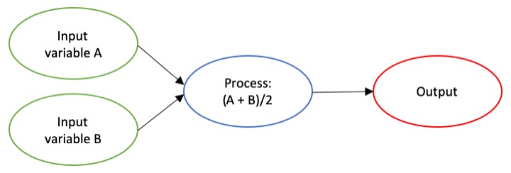
The dictionary broadly defines an algorithm as “a step-by-step procedure for solving a problem or accomplishing some end” (Merriam-Webster). Imagine an algorithm as a flow chart (Fig. 1), where each step is some process that is applied to the input(s) to get the desired output. In image analysis the output is usually isolated sections of the image that represent a specific feature; for example, isolating and counting the number of penguins in an image. Algorithm development involves figuring out which processes to use in order to consistently get desired results. I have conducted image analysis previously and these processes typically involve figuring out how to find a certain cutoff value. But, before I go too far down that road, let’s break down an image and the characteristics that are important for image analysis.

Figure 1. An example of a basic algorithm flow chart. There are two inputs: variables A and B. The process is the calculation of the mean of the two variables.

What is an image?

Think of an image as a spread sheet, where each cell is a pixel and each pixel is assigned a value (Fig. 2). Each value is associated with a color and when the sheet is zoomed out and viewed as a whole, the image comes together.  In color imagery, which is also referred to as RGB, each pixel is associated with the values of the three color bands (red, green, and blue) that make up that color. In a thermal image, each pixel’s value is a temperature value. Thinking about an image as a grid of values is helpful to understand the challenge of translating the larger patterns we see into something the computer can interpret. In image analysis this process can involve using the values of the pixels themselves or the relationships between the values of neighboring pixels.

Figure 2. A diagram illustrating how pixels make up an image. Each pixel is a grid cell associated with certain values. Image Source: https://web.stanford.edu/class/cs101/image-1-introduction.html

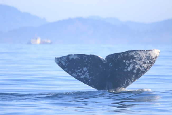
Our brains take in the whole picture at once and we are good at identifying the objects and patterns in an image. Take Figure 3 for example: an astute human eye and brain can isolate and identify all the different markings and scars on the fluke. Yet, this process would be very time consuming. The trick to building an algorithm to conduct this work is figuring out what processes or tools are needed to get a computer to recognize what is marking and what is not. This iterative process is the algorithm development.

Figure 3. Photo ID image of a gray whale fluke.

Development

An image analysis algorithm will typically involve some sort of thresholding. Thresholds are used to classify an image into groups of pixels that represent different characteristics. A threshold could be applied to the image in Figure 3 to separate the white color of the markings on the fluke from the darker colors in the rest of the image. However, this is an oversimplification, because while it would be pretty simple to examine the pixel values of this image and pick a threshold by hand, this threshold would not be applicable to other images. If a whale in another image is a lighter color or the image is brighter, the pixel values would be different enough from those in the previous image for the threshold to inaccurately classify the image. This problem is why a lot of image analysis algorithm development involves creating parameterized processes that can calculate the appropriate threshold for each image.

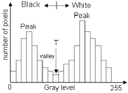
One successful method used to determine thresholds in images is to first calculate the frequency of color in each image, and then apply the appropriate threshold. Fletcher et al. (2009) developed a semiautomated algorithm to detect scars in seagrass beds from aerial imagery by applying an equation to a histogram of the values in each image to calculate the threshold. A histogram is a plot of the frequency of values binned into groups (Fig. 4). Essentially, it shows how many times each value appears in an image. This information can be used to define breaks between groups of values. If the image of the fluke were transformed to a gray scale, then the values of the marking pixels would be grouped around the value for white and the other pixels would group closer to black, similar to what is shown in Figure 4. An equation can be written that takes this frequency information and calculates where the break is between the groups. Since this method calculates an individualized threshold for each image, it’s a more reliable method for image analysis. Other characteristics could also be used to further filter the image, such as shape or area.

However, that approach is not the only way to make an algorithm applicable to different images; semi-automation can also be helpful. Semi-automation involves some kind of user input. After uploading the image for analysis, the user could also provide the threshold, or the user could crop the image so that only the important components were maintained. Keeping with the fluke example, the user could crop the image so that it was only of the fluke. This would help reduce the variety of colors in the image and make it easier to distinguish between dark whale and light marking.

Figure 4. Example histogram of pixel values. Source: Moallem et al. 2012

Why algorithms are important

Algorithms are helpful because they make our lives easier. While it would be possible for an analyst to identify and digitize each individual marking from a picture of a gray whale, it would be extremely time consuming and tedious. Image analysis algorithms significantly reduce the time it takes to process imagery. A semi-automated algorithm that I developed to count penguins from still drone imagery can count all the penguins on a one km2 island in about 30 minutes, while it took me 24 long hours to count them by hand (Bird et al. in prep). Furthermore, the process can be repeated with different imagery and analysts as part of a time series without bias because the algorithm eliminates human error introduced by different analysts.

Whether it’s a simple combination of a few processes or a complex series of equations, creating an algorithm requires breaking down a task to its most basic components. Development involves translating those components step by step into an automated process, which after many trials and errors, achieves the desired result. My first algorithm project took two years of revising, improving, and countless trials and errors.  So, whether creating an algorithm or working to understand one, don’t let the jargon nor the endless trials and errors stop you. Like most things in life, the key is to have patience and take it one step at a time.

References

Bird, C. N., Johnston, D.W., Dale, J. (in prep). Automated counting of Adelie penguins (Pygoscelis adeliae) on Avian and Torgersen Island off the Western Antarctic Peninsula using Thermal and Multispectral Imagery. Manuscript in preparation

Fletcher, R. S., Pulich, W. ‡, & Hardegree, B. (2009). A Semiautomated Approach for Monitoring Landscape Changes in Texas Seagrass Beds from Aerial Photography. https://doi.org/10.2112/07-0882.1

Moallem, Payman & Razmjooy, Navid. (2012). Optimal Threshold Computing in Automatic Image Thresholding using Adaptive Particle Swarm Optimization. Journal of Applied Research and Technology. 703.

Robots are taking over the oceans

By Leila Lemos, PhD Student

In the past few weeks I read an article on the use of aquatic robots in the ocean for research. Since my PhD project uses technology, such as drones and GoPros, to monitor body condition of gray whales and availability of prey along the Oregon coast, I became really interested by the new perspective these robots could provide. Drones produce aerial images while GoPros generate an underwater-scape snapshot. The possible new perspective provided by a robot under the water could be amazing and potentially be used in many different applications.

The article was published on March 21st by The New York Times, and described a new finned robot named “SoFi” or “Sophie”, short for Soft Robotic Fish (Figure 1; The New York Times 2018). The aquatic robot was designed by scientists at the Massachusetts Institute of Technology (MIT) Computer Science and Artificial Intelligence Lab, with the purpose of studying marine life in their natural habitats.

Figure 1: “SoFi”, a robotic fish designed by MIT scientists.
Source: The New York Times 2018.


SoFi’s  first swim trial occurred in a coral reef in Fiji, and the footage recorded can be seen in the following video:


SoFi can swim at depths up to 18 meters and at speeds up to half-its-body-length a second (average of 23.5 cm/s in a straight path; Katzschmann et al. 2018). Sofi can swim for up to ~40 minutes, as limited by battery time. The robot is also well-equipped (Figure 2). It has a compact buoyancy control mechanism and includes a wide-view video camera, a hydrophone, a battery, environmental sensors, and operating and communication systems. The operating and communication systems allow a diver to issue commands by using a controller that operates through sound waves.

Figure 2: “SoFi” system subcomponents overview.
Source: Katzschmann et al. 2018.


The robot designers highlight that while SoFi was swimming, fish didn’t seem to be bothered or get scared by SoFi’s presence. Some fish were seen swimming nearby the robot, suggesting that SoFi has the potential to integrate into the natural underwater environment and therefore record undisturbed behaviors. However, a limitation of this invention is that SoFi needs a diver on scene to control the robot. Therefore, SoFi’s study of marine life without human interference may be compromised until technology develops further.

Another potential impact of SoFi we might be concerned about is noise. Does this device produce noise levels that marine fauna can sense or maybe be stress by? Unfortunately, the answer is yes. Even if fish don’t seem to be bothered by SoFi’s presence, it might bother other animals with hearing sensitivity in the same frequency range of SoFi. Katzschmann and colleagues (2018) explained that they chose a frequency to operate SoFi that would minimally impact marine fauna. They studied the frequencies used by the aquatic animals and, since the hearing ranges of most aquatic species decays significantly above 10 KHz, they selected a frequency above this range (i.e., 36 KHz). However, this high frequency range can be sensed by some species of cetaceans and pinnipeds, but negative affects on these animals will be dependent on the sound amplitude that is produced.

Although not perfect (but what tool is?), SoFi can be seen as a great first step toward a future of underwater robots to assist research efforts.  Battery life, human disturbance, and noise disturbance are limitations, but through thoughtful application and continued innovation this fishy tool can be the start of something great.

The use of aquatic robots, such as SoFi, can help us advance our knowledge in underwater ecosystems. These robots could promote a better understanding of marine life in their natural habitat by studying behaviors, interactions and responses to threats. These robots may offer important new tools in the protection of animals against the effects caused by anthropogenic activities. Additionally, the use of aquatic robots in scientific research may substitute remote operated vehicles and submersibles in some circumstances, such as how drones are substituting for airplanes sometimes, thus providing a less expensive and better-tolerated way of monitoring wildlife.

Through continued multidisciplinary collaboration by robot designers, biologists, meteorologists, and more, innovation will continue allowing data collection with minimal to non-disturbance to the wildlife, providing lower costs and higher safety for the researchers.

It is impressive to see how technology efforts are expanding into the oceans. As drones are conquering our skies today and bringing so much valuable information on wildlife monitoring, I believe that the same will occur in our oceans in a near future, assisting in marine life conservation.


References:

Katzschmann RK, DelPreto J, MacCurdy R, Rus D. 2018. Exploration of Underwater Life with an Acoustically Controlled Soft Robotic Fish. Sci. Robot. 3, eaar3449. DOI: 10.1126/scirobotics.aar3449.

The New York Times. 2018. Robotic Fish to Keep a Fishy Eye on the Health of the Oceans. Available at: https://www.nytimes.com/2018/03/21/science/robot-fish.html.

Coastal oceanography takes patience

Joe Haxel, Acoustician, Assistant Professor, CIMRS/OSU

Greetings GEMM Lab blog readers. My name is Joe Haxel and I’m a close collaborator with Leigh and other GEMM lab members on the gray whale ecology, physiology and noise project off the Oregon coast. Leigh invited me for a guest blog appearance to share some of the acoustics work we’ve been up to and as you’ve probably guessed by now, my specialty is in ocean acoustics. I’m a PI in NOAA’s Pacific Marine Environmental Laboratory’s Acoustics Program and OSU’s Cooperative Institute for Marine Resources Studies where I use underwater sound to study a variety of earth and ocean processes.

As a component of the gray whale noise project, during the field seasons of 2016 and 2017 we recorded some of the first measurements of ambient sound in the shallow coastal waters off Oregon between 7 and 20 meters depth. In the passive ocean acoustics world this is really shallow, and with that comes all kinds of instrument and logistical challenges, which is probably one of the main reasons there is little or no acoustic baseline information in this environment.

For instance, one of the significant challenges is rooted in the hydrodynamics surrounding mobile recording systems like the drifting hydrophone we used during the summer field season in 2016 (Fig 1). Decoupling motion of the surface buoy (e.g., caused by swell and waves) from the submerged hydrophone sensor is critical, and here’s why. Hydrophones convert pressure fluctuations at the sensor/ water interface to a calibrated voltage recorded by a logging system. Turbulence resulting from moving the sensor up and down in the water column with surface waves introduces non-acoustic pressure changes that severely contaminate the data for noise level measurements. Vertical and horizontal wave motions are constantly acting on the float, so we needed to engineer compliance between the surface float and the suspended hydrophone sensor to decouple these accelerations. To overcome this, we employed a couple of concepts in our drifting hydrophone design. 1) A 10 cm diameter by 3 m long spar buoy provided floatation for the system. Spar buoys are less affected by wave motion accelerations compared to most other types of surface floatation with larger horizontal profiles and drag. 2) A dynamic shock cord that could stretch up to double its resting length to accommodate vertical motion of the spar buoy; 3) a heave plate that significantly reduced any vertical motion of the hydrophone suspended below it. This was a very effective design, and although somewhat cumbersome in transport with the RHIB between deployment sites, the acoustic data we collected over 40 different drifts around Newport and Port Orford in 2016 was clean, high quality and devoid of system induced contamination.

Figure 1. The drifting hydrophone system used for 40 different drifts recording ambient noise levels in 7-20 m depths in the Newport and Port Orford, OR coastal areas.


Spatial information from the project’s first year acoustic recordings using the drifting hydrophone system helped us choose sites for the fixed hydrophone stations in 2017. Now that we had some basic information on the spatial variability of noise within the study areas we could focus on the temporal objectives of characterizing the range of acoustic conditions experienced by gray whales over the course of the entire foraging season at these sites in Oregon. In 2017 we deployed “lander” style instrument frames, each equipped with a single, omni-directional hydrophone custom built by Haru Matsumoto at our NOAA/OSU Acoustics lab (Fig. 2). The four hydrophone stations were positioned near each of the ports (Yaquina Bay and Port Orford) and in partnership with the Oregon Department of Fish and Wildlife Marine Reserves program in the Otter Rock Marine Reserve and the Redfish Rocks Marine Reserve. The hydrophones were programmed on a 20% duty cycle, recording 12 minutes of every hour at 32 kHz sample rate, providing spectral information in the frequency band from 10 Hz up to a 13 kHz.

Figure 2. The hydrophone (black cylinder) on its lander frame ready for deployment.

Here’s where the story gets interesting. In my experience so far putting out gear off the Oregon coast, anything that has a surface expression and is left out for more than a couple of weeks is going to have issues. Due to funding constraints, I had to challenge that theory this year and deploy 2 of the units with a surface buoy. This is not typically what we do with our equipment since it usually stays out for up to 2 years at a time, is sensitive, and expensive. The 2 frames with a surface float were going to be deployed in Marine Reserves far enough from the traffic lanes of the ports and in areas with significantly less traffic and presumably no fishing pressure.  The surface buoy consisted of an 18 inch diameter hard plastic float connected to an anchor that was offset from the instrument frame by a 150 foot weighted groundline. The gear was deployed off Newport in June and Port Orford in July. What could go wrong?

After monthly buoy checks by the project team, including GPS positions, and buoy cleanings my hopes were pretty high that the surface buoy systems might actually make it through the season with recoveries scheduled in mid-October. Had I gambled and won? Nope. The call came in September from Leigh that one of the whale watching outfits in Depoe Bay recovered a free floating buoy matching ours. Bummer. Alternative recovery plans initiated and this is where things began to get hairy. Fortunately, we had an ace in our back pocket. We have collaborators at the Oregon Coast Aquarium (OCA) who have a top-notch research diving team led by Jim Burke. In the last week of October, they performed a successful search dive on the missing unit near Gull Rock and attached a new set of floats directly to the instrument frame. The divers were in the water for a short 20 minutes thanks to the good series of marks recorded during the buoy checks throughout the summer (Fig. 3).

Figure 3. OCA divers, Jenna and Doug, heading out for a search dive to locate and mark the Gull Rock hydrophone lander.


We had surface marker floats on the frame, but there was a new problem. Video taken by Jenna and Doug from the OCA dive team revealed the landers were pretty sanded in from a couple of recent October storms (Fig. 4). Ugghhh!

Figure 4. Sanded in lander at Gull Rock. Notice the sand dollars and bull kelp wrapped on the frame.

Alternative recovery plan adjustment: we’re gonna need a diver assisted recovery with 2 boats. One to bring a dive team to air jet the sand out away from the legs of the frame and another larger vessel with pulling power to recover the freed lander. Enter the R/V Pacific Surveyor and Capt. Al Pazar. Al, Jim and I came up with a new recovery plan and only needed a decent weather window of a few hours to get the job done. Piece of cake in November off the Oregon coast, right?

The weather finally cooperated in early December in-line with the OCA dive team and R/V Pacific Surveyor’s availability. The 2 vessels and crew headed up to Gull Rock for the first recovery operation of the day. At first we couldn’t locate the surface floats. Oh no. It seemed the rough fall/ winter weather and high seas since late October were too much for the crab floats? As it turns out, we eventually found the floats eastward about 200 m but couldn’t initially see them in the glare and whitecapping conditions that morning. The lander frame had broken loose from its weakened anchor legs in the heavy weather (as it was designed to do through an Aluminum/ Stainless Steel galvanic reaction over time) and rolled or hopped eastward by about 200 m (Fig. 5). Oh dear!

Figure 5. A hydrophone lander after recovery. Notice all but 1 of the concrete anchor legs missing from the recovered lander and the amount of bio-fouling on the hydrophone (compared to Figure 2).


Thankfully, the hydrophone was well protected, and no air jetting was required. With OCA divers out of the water and clear, the Pacific Surveyor headed over to the floats and easily pulled the lander frame and hydrophone on board (Fig. 6). Yipee!

On to the next hydrophone station. This station, deployed ~ 800 m west of the south reef off of South Beach near the Yaquina Bay port entrance. It was deployed entirely subsurface and was outfitted with an acoustic release transponder that I could communicate with from the surface and command to release a pop-up messenger float and line for eventual recovery of the instrument frame. Once on station, communication with the release was established easily (a good start) and we began ranging and moving the OCA vessel Gracie Lynn in to a position within about 2 water depths of the unit (~40 m). I gave the command to the transponder and the submerged release confirmed it was free of its anchor and heading for the surface, but it never made it. Uh oh. Turns out this lander had also broke free of its anchored legs and rolled/ hopped 800 m eastward until it was pinned up against the boulder structure of the south reef. Amazingly, OCA divers Jenna and Doug located the messenger float ~ 5 m below the surface and the messenger line had been fouled by the rolling frame so it could not reach the surface. They dove down the messenger line and attached a new recovery line to the lander frame and the Pacific Surveyor hauled up the frame and hydrophone in-tact (Fig. 6). Double recovery success!

Figure 6. R/V Pacific Surveyor recovering hydrophone landers off Gull Rock and South Beach.

The hydrophone data from both systems looks outstanding and analysis is underway. This recovery effort took a huge amount of patience and the coordination of 3 busy groups (NOAA/OSU, OCA, Capt. Al). Thanks to these incredible collaborations and some heroic diving from Jim Burke and his OCA dive team, we now have a unique and unprecedented shallow water passive acoustic data set from the energetic waters off the Oregon coast.

So that’s some of the story from the 2016 and 2017 field season acoustic point of view. I’ll save the less exciting, but equally successful instrument recoveries from Port Orford for another time.

From the highs to the lows, that’s just how it blows!


By: Kelli Iddings, MSc Student, Duke University, Nicholas School of the Environment

The excitement is palpable as I wait in anticipation. But finally, “Blow!” I shout as I notice the lingering spray of seawater expelled from a gray whale as it surfaces to breathe. The team and I scurry about the field site taking our places and getting ready to track the whale’s movements. “Gray whale- Traveling- Group 1- Mark!” I exclaim mustering enough self-control to ignore the urge to drop everything and stand in complete awe of what in my mind is nothing short of a miracle. I’ve spotted a gray whale searching and foraging for food! As a student of the Master of Environmental Management program at Duke University, I am collaborating on a project in Port Orford, Oregon where my team and I are working to gain a better understanding of the interactions between the Pacific Coast Feeding Group (PCFG) gray whales and their prey. Check out this blog post written earlier by my teammate Florence to learn more about the methods of the project and what motivated us to take a closer look at the foraging behavior of this species.

Understanding the dynamics of gray whale foraging within ecosystems where they are feeding is essential to paint a more comprehensive picture of gray whale health and ecology—often with the intent to protect and conserve them. A lot of our recent effort has been focused on developing and testing methods that will allow us to answer the questions that we are asking. For example, what species of prey are the PCFG whales feeding on in Port Orford? Based on the results of a previous study (Newell and Cowles 2006) that was conducted in Depoe Bay, Oregon, and a lot of great knowledge from the local fisheries and the Port Orford community, we hypothesized that the whales were feeding on a small, shrimp-like crustacean in the order Mysida. Given the results of our videos, and the abundance of mysid, it looks like we are right (Fig. 1)!

DSCF0776[3]
Figure 1: Mysids, only 5-25mm in length, collected in Tichenor Cove using a downrigger to lower a weighted plankton net into the water column from our kayak.
Mysids are not typically the primary food source of gray whales. In their feeding grounds in the Bering and Chukchi Seas near Alaska, the whales feed on benthic amphipods on the ocean floor by sucking up sediment and water and pushing it through baleen plates that trap the food as the water and sediment is filtered out. However, gray whales demonstrate flexible feeding strategies and are considered opportunistic feeders, meaning they are not obligate feeders on one prey item like krill-dependent blue whales. In Oregon, mysid congregate in dense swarms by the billions, which we hypothesize, makes it energetically worthwhile for the massive 13-15m gray whales to hang around and feed! Figure 2 illustrates a mysid swarm of this kind in Tichenor Cove.

DCIM102GOPROG0132732.
Figure 2: Image captured using a Hero 4 Black GoPro. Rocky Substrate is visible in lower portion of image and a clear swarm of mysid is aggregated around this area.

Once we know what the gray whales are eating, and why, we ask follow up questions like how is the distribution of mysid changing across space and time, if at all? Are there patterns? If so, are the patterns influencing the feeding behavior and movement of the whales? For the most part, we are having success characterizing the relative abundances of mysid. No conclusions can be made yet, but there are a few trends that we are noticing. For instance, it seems that the mysid are, as we hypothesized, very dense and abundant around the rocky shoreline where there are kelp beds. Could these characteristics be predictors of critical habitat that whales seek as foraging grounds? Is it the presence of kelp that mysid prefer? Or maybe it’s the rocky substrate itself? Distance to shore? Time and data analysis will tell. We have also noticed that mysid seem to prefer to hang out closer to the bottom of the water column. Last, but certainly not least, we are already noticing differences in the sizes and life stages of the mysid over the short span of one week at our research site! We are excited to explore these patterns further.

The biggest thing we’re learning out here, however, is the absolute necessity for patience, ingenuity, adaptability, and perseverance in science. You heard that right, as with most things, I am learning more from our failures, than I am from our successes.  For starters, understanding mysid abundance and distribution is great in and of itself, but we cannot draw any conclusions about how those factors are affecting whales if the whales don’t come! We were very fortunate to see whales while training on our instruments in Newport, north of our current study site. We saw whales foraging, whales searching, mother/calf pairs, and even whales breaching! Since we’ve been in Port Orford, we have seen only three whales, thrown in among the long hours of womanpower (#WomenInScience) we have been putting in! We are now learning the realities of ecological science that >gasp< fieldwork can be boring! Nevertheless, we trust that the whales will hear our calls (Yes, our literal whale calls. Like I said, it can get boring up on the cliff) and head on over to give the cliff team in Port Orford some great data—and excitement!

Then, there is the technology. Oh, the joys of technology. You see I’ve never considered myself a “techie.” Honestly, I didn’t even know what a hard drive was until some embarrassing time in the not-so-distant past. And now, here I am working on a project that is using novel, technology rich approaches to study what I am most passionate about. Oh, the irony. Alas, I have been putting on my big girl britches, saddling up, and taking the whale by the fluke. Days are spent syncing a GoPro, Time-Depth Recorder (TDR), GPS, associated software, and our trusty rugged laptop, all the while navigating across multiple hard drives, transferring and organizing massive amounts of data, reviewing and editing video footage, and trouble shooting all of it when something, inevitably, crashes, gets lost, or some other form of small tragedy associated with data management. Sounds fun, right? Nonetheless, within the chaos and despair, I realize that technology is my friend, not my foe. Technology allows us to collect more data than ever before, giving us the ability to see trends that we could not have seen otherwise, and expending much less physical effort doing so. Additionally, technology offers many alternatives to other invasive and potentially destructive methods of data collection. The truth is if you’re not technologically savvy in science these days, you can expect to fall behind. I am grateful to have an incredible team of support and such an exciting project to soften the blow. Below (Fig. 3) is a picture of myself embracing my new friend technology.

DSCF0758
Figure 3: Retrieving the GoPro, and some tag-a-long kelp, from the water after a successful deployment in Tichenor Cove.

Last but not least, there are those moments that can best be explained by the Norwegian sentiment “Uff da!” I was introduced to the expression while dining at The Crazy Norwegian, known famously for having the best fish and chips along the entire west coast and located dangerously close to the field station. The expression dates back to the 19th century, and is used readily to concisely convey feelings of surprise, astonishment, exhaustion, and sometimes dismay. This past week, the team was witness to all of these feelings at once as our GoPro, TDR, and data fell swiftly to the bottom of the 42-degree waters of Tichenor cove after the line snapped during deployment. Uff da!!! With our dive contact out of town, red tape limiting our options, the holiday weekend looming ahead, and the dreadful thought of losing our equipment on a very tight budget, the team banded together to draft a plan. And what a beautiful plan it was! The communities of Port Orford, Oregon State University, and the University of Oregon’s Institute of Marine Biology came together in a successful attempt to retrieve the equipment. We offer much gratitude to Greg Ryder, our retrieval boat operator, OSU dive safety operator Kevin Buch, and our divers, Aaron Galloway and Taylor Eaton! After lying on the bottom of the cove for almost three days, the divers retrieved our equipment within 20 minutes of the dive – thanks to the quick and mindful action of our kayak team to mark a waypoint on the GPS at the time of the equipment loss. Please enjoy this shot (Fig. 4) of Aaron and Taylor surfacing with the gear as much as we do!

Figure 4: Aaron Galloway and Taylor Eaton surface with our lost piece of equipment after a successful dive retrieval mission.

The moral of the story is that science isn’t easy, but it’s worth it. It takes hard work, long hours, frustration, commitment, collaboration, and preparedness. But moments come along when your team sits around a dining room table, exhausted from waking and paddling at 5 am that morning, and continues to drive forward. You creatively brainstorm, running on the fumes of the passion and love for the ocean and creatures within it that brought everyone together in the first place; each person growing in his or her own right. Questions are answered, conclusions are drawn, and you go to bed at the end of it all with a smile on your face, anxiously anticipating the little miracles that the next day’s light will bring.

References

Newell, C. and T.J. Cowles. (2006). Unusual gray whale Eschrichtius robustus feeding in the summer of 2005 off the central Oregon Coast. Geophysical Research Letters, 33:10.1029/2006GL027189