Baleen analyses reveals patterns in foraging ecology and stress physiology in gray whales prior to death.

Dr. Alejandro A. Fernández Ajó, Postdoctoral Scholar, Marine Mammal Institute – OSU Department of Fisheries, Wildlife, & Conservation Sciences, Geospatial Ecology of Marine Megafauna (GEMM) Lab.

The Eastern North Pacific (ENP) gray whale population has experienced at least two recorded Unusual Mortality Events (UMEs), from 1999–2000 and from 2019 to 2024, during which many gray whales stranded along the Pacific coast from northern Mexico to the Alaskan Arctic, USA (Martínez-Aguilar et al., 2019; Urbán, 2020). Several factors have been considered as possible causes for the high number of gray whale’s strandings, including variation in Arctic prey availability and the duration of their feeding season caused by the timing of sea ice formation and breakup (Stewart et al., 2023), starvation, anthropogenically derived toxicants, biotoxins, infectious diseases, parasites, fisheries interactions, and ship strikes (F. Gulland et al., 2005). In the most recent UME, many of the stranded whales showed signs of emaciation, indicating malnutrition as a causal factor of death (Christiansen et al., 2021; Torres et al., 2022). While the poor condition of many of the stranded whales supports the idea of starvation as a cause for these mortalities, the underlying causes of malnutrition are unknown, and it is also unclear whether the whales’ decline in body condition was rapid or gradual.

Figure 1. Gray whale with baleen exposed. Photo: GEMM Lab  NOAA/NMFS permit #16111.

Large whales face a multitude of stressors in their environment, ranging from ocean noise to contaminants, climate change, and prey shifts. Understanding how individual whales respond to these disturbances is crucial for assessing potential impacts on the population as a whole. However, monitoring the health parameters and vital rates of whales presents significant challenges due to their large size, mobility, and the vast ranges of their marine habitat. Studying stranded whales can provide valuable insights into health risks, disease susceptibility, and the impacts of pollutants and other stressors on whale populations, thus informing conservation strategies (see post). Nonetheless, the quality of information obtained from necropsies heavily relies on the timeliness of stranding reports, as decomposition begins immediately after death, limiting detailed investigations into the cause of death. Therefore, establishing a robust network capable of promptly reporting and addressing stranding events is essential (Gulland & Stockin, 2020). An effective network involves having well-trained staff, proper infrastructure, sufficient funding, and the expertise and tools necessary to gather and analyze data and samples to infer their health and causes of mortality.

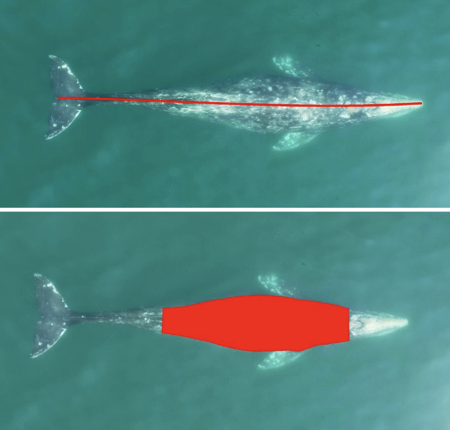
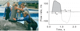
During my doctoral dissertation, I worked to develop and ground truth the endocrine analyses of whale baleen as a novel sample type that can be used for retrospective assessments of the whale’s physiology (see my previous post & post). Baleen, the filter-feeding apparatus of mysticetes whales (Figure 1), consists of long fringed plates of keratinized tissue that grow continuously and slowly downward from the whale’s upper jaw. These plates are routinely collected at necropsies; and unlike other tissue types, they are durable and have minimum storage requirements; they can be preserved dry at room temperature, allowing for the analysis of both historical and current whale populations. Moreover, while most sample types used for studying whale health and physiology provide a single time-point measure of current circulating hormone levels (e.g., skin or respiratory vapor) or hold integrated information from the previous few hours or days (e.g., urine and feces), baleen tissue provides a unique opportunity for retrospective and longitudinal analyses of multiple biological parameters of the individual during the time that the tissue was grown, i.e., months to years prior to death, helping to describe the whale’s physiology, migration patterns, and exposure to pollutants (see my previous post).

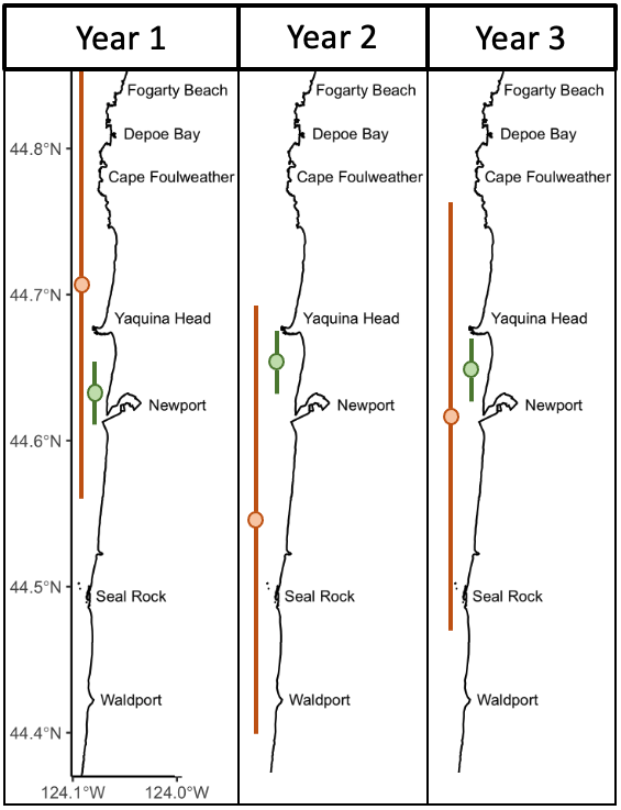
In our recent study, “A longitudinal study of endocrinology and foraging ecology of subadult gray whales prior to death based on baleen analysis”, published in the journal General and Comparative Endocrinology, we examine isotope and hormone levels in the baleen of five young gray whales stranded in central Oregon during the most recent UME. Our primary objectives were to retrospectively examine the hormone and isotopic profiles of the individual whales prior to mortality, assess potential factors contributing to death, and identify the timing for the onset of chronic illness leading to mortality. Our analysis included tracing longitudinal changes in (1) stable isotope values in baleen (δ13C and δ15N), which allowed us to infer the baleen growth rate and assess the seasonal changes in diet and foraging location in large whales (Figure 2), along with the quantification of (2) two adrenal glucocorticoid steroids that are biomarkers for the whale’s stress response, (3) one thyroid hormone (triiodothyronine, T3) as an indicator of nutritional state, and (4) two sex hormones, progesterone and testosterone, to infer about reproductive status and sexual maturity. By integrating isotopic and hormonal methodologies, our study demonstrates how baleen analysis offers a comprehensive narrative of the endocrine and trophic ecology of individual whales over time.

Figure 2. Gray whales, like other large marine mammals that rely on built-up energy reserves, exhibit distinct seasonal shifts in their feeding habits. During summer, these whales feed at the ocean’s bottom, consuming organisms lower in the food chain, which is reflected in lower nitrogen values in their baleen (summer foraging). In winter, however, they must rely on their own fat reserves, causing an increase in nitrogen values (wintering). In this plot we can observe the oscillations in δ15N over time; this information allows us to estimate the baleen growth rate. Our results suggest that gray whale baleen holds a record of around 1.3 years of stable isotopes and hormone data prior to the time of death (Fernandez Ajo et al. 2024). The red cross in the X-axis, indicate the time of death. Gray whale illustration https://www.fisheries.noaa.gov/species/gray-whale

Our endocrine assessments revealed detailed profiles of stress-related hormones (glucocorticoids, cortisol) and thyroid hormones along the lengths of the baleen. We found increased levels of cortisol in whales that died from unknown causes, starting about eight months prior to their deaths. This suggests these whales were under prolonged stress before dying. In contrast, in the case of a whale killed acutely by a killer whale, cortisol levels were low and constant prior to death, indicating this individual was likely in good health prior to the sudden attack. In terms of thyroid activity, indicated by T3 hormone levels, we found a gradual increase over several months in the whales that died of unknown causes. This pattern is not typically expected, as stress usually suppresses thyroid function. This anomaly could suggest an adaptive response to maintain body temperature and metabolism in potentially malnourished whales. Regarding the sex hormones, as expected for this age class, we found no significant fluctuations or spikes that would indicate sexual maturity in these young whales (Figure 3).

Figure 3. Longitudinal hormone profiles in an individual gray whale that died due to unknown causes (left) and one that died acutely due to orca predation (right). Note the pronounced elevations in cortisol levels (indicative of stress) and T3 prior to death in the case of unknown cause of death, while hormone levels remained low and constant prior to death in the whale acutely killed. Sex hormones do not present any clear oscillations, indicating that these whales were likely sexually immature. The red cross in the X-axis, indicate the time of death. Killer whale (Orcinus orca) illustration https://www.fisheries.noaa.gov/species/ killer-whale

Although commercial whaling is currently banned and several whale populations show evidence of recovery, today’s whales are exposed to a variety of other human stressors that cause significant lethal and non-lethal impacts (e.g., entanglement in fishing gear, vessel strikes, shipping noise, climate change, etc.; reviewed in Thomas et al., 2016). The recovery and conservation of large whale populations is particularly important to the oceanic environment due to their key ecological role and unique biological traits (See my previous post). Our research demonstrates the strengths of using baleen as a tool for the retrospective assessments of whale endocrinology and trophic ecology. As the Eastern North Pacific gray whale population faces recurring challenges, indicated by fluctuating numbers and unusual mortality events, innovative techniques like the baleen analysis presented here, are essential to investigate the causes of mortality and inform management, helping us understand not only the immediate causes of death but also broader environmental and ecological changes affecting their survival. Broadly implementing this approach with a greater sample size of baleen collected across a larger spatial and temporal range could significantly improve our strategies for conservation and management of baleen whales.

Did you enjoy this blog? Want to learn more about marine life, research, and
conservation? Subscribe to our blog and get a weekly message when we post a new
blog. Just add your name and email into the subscribe box below.

Loading

References

Christiansen, F., Rodríguez-González, F., Martínez-Aguilar, S., Urbán, J., Swartz, S., Warick, H., Vivier, F., & Bejder, L. (2021). Poor body condition associated with an unusual mortality event in gray whales. Marine Ecology Progress Series, 658, 237–252. https://doi.org/10.3354/meps13585

Gulland, F. M. D., & Stockin, K. A. (2020). Harmonizing global strandings response. European Cetacean Society Special Publication Series.

Gulland, F., Pérez-Cortés, H., Urbán, J. R., Rojas-Bracho, L., Ylitalo, G., Weir, J., Norman, S., Muto, M., Rugh, D., Kreuder, C., & Rowles, T. (2005). Eastern North Pacific gray whale (Eschrichtius robustus) unusual mortality event, 1999-2000. U.S. Department of Commerce. NOAA Technical Memorandum. NMFS-AFSC-150., March, 33 pp. http://www.afsc.noaa.gov/publications/AFSC-TM/NOAA-TM-AFSC-150.pdf

Martínez-Aguilar, S., Mariano-Meléndez, E., López-Paz, N., Castillo-Romero, F., Zaragoza-aguilar, G. A., Rivera-Rodriguez, J., Zaragoza-Aguilar, A., Swartz, S., Viloria-Gómora, L., & Urbán, J. R. (2019). Gray whale (Eschrichtius robustus) stranding records in Mexico during the winter breeding season in 2019. Report of the International Whaling Commission. Document SC/68A/CMP/14, May.

Stewart, J. D., Joyce, T. W., Durban, J. W., Calambokidis, J., Fauquier, D., Fearnbach, H., Grebmeier, J. M., Lynn, M., Manizza, M., Perryman, W. L., Tinker, M. T., & Weller, D. W. (2023). Boom-bust cycles in gray whales associated with dynamic and changing Arctic conditions. Science, 382(6667), 207–211. https://doi.org/10.1126/science.adi1847

Torres, L. G., Bird, C. N., Rodríguez-González, F., Christiansen, F., Bejder, L., Lemos, L., Urban R, J., Swartz, S., Willoughby, A., Hewitt, J., & Bierlich, KC. (2022). Range-Wide Comparison of Gray Whale Body Condition Reveals Contrasting Sub-Population Health Characteristics and Vulnerability to Environmental Change. Frontiers in Marine Science, 9. https://doi.org/10.3389/fmars.2022.867258

Urbán, R. (2020). Gray whale stranding records in Mexico during the 2020 winter breeding season. Unpublished Paper SC/68B/CMP/13 Presented to the IWC Scientific Committee, Cambridge.

An ‘X’travaganza! Introducing the Marine Mammal Institute’s Center of Drone Excellence (CODEX)

Dr. KC Bierlich, Postdoctoral Scholar, OSU Department of Fisheries, Wildlife, & Conservation Sciences, Geospatial Ecology of Marine Megafauna Lab

Drones are becoming more and more prevalent in marine mammal research, particularly for non-invasively obtaining morphological measurements of cetaceans via photogrammetry to identify important health metrics (see this and this previous blog). For example, the GEMM Lab uses drones for the GRANITE Project to study Pacific Coast Feeding Group (PCFG) gray whales and we have found that PCFG whales are skinnier and morphologically shorter with smaller skulls and flukes compared to the larger Eastern North Pacific (ENP) population. The GEMM Lab has also used drones to document variation in body condition across years and within a season, to diagnose pregnancy, and even measure blowholes.

While drone-based photogrammetry can provide major insight into cetacean ecology, several drone systems and protocols are used across the scientific community in these efforts, and no consistent method or centralized framework is established for quantifying and incorporating measurement uncertainty associated with these different drones. This lack of standardization restricts comparability across datasets, thus hindering our ability to effectively monitor populations and understand the drivers of variation (e.g., pollution, climate change, injury, noise).

We are excited to announce the Marine Mammal Institute’s (MMI) Center of Drone Excellence (CODEX), which focuses on developing analytical methods for using drones to non-invasively monitor marine mammal populations. CODEX is led by GEMM Lab member’s KC Bierlich, Leigh Torres, and Clara Bird and consists of other team members within and outside OSU. We draw from many years of trials, errors, headaches, and effort working with drones to study cetacean ecology in a variety of habitats and conditions on many different species.

Already CODEX has developed several open-source hardware and software tools. We developed, produced, and published LidarBoX (Bierlich et al., 2023), which is a 3D printed enclosure for a LiDAR altimeter system that can be easily attached and swapped between commercially available drones (i.e., DJI Inspire, DJI Mavic, and DJI Phantom) (Figure 1). Having a LidarBoX installed helps researchers obtain altitude readings with greater accuracy, yielding morphological measurements with less uncertainty. Since we developed LidarBoX, we have received over 35 orders to build this unit for other labs in national and international universities.

Figure 1. A ‘LidarBoX’ attached to a DJI Inspire 2. The LidarBoX is a 3D printed enclosure containing a LiDAR altimeter to help obtain more accurate altitude readings.

Additionally, CODEX recently released MorphoMetriX version 2 (v2), an easy-to-use photogrammetry software that provides users with the flexibility to obtain custom morphological measurements of megafauna in imagery with no knowledge of any scripting language (Torres and Bierlich, 2020). CollatriX is a user-friendly software for collating multiple MorphoMetriX outputs into a single dataframe and linking important metadata to photogrammetric measurements, such as altitude measured with a LidarBoX (Bird and Bierlich, 2020). CollatriX also automatically calculates several body condition metrics based on measurements from MorphoMetriX v2. CollatriX v2 is currently in beta-testing and scheduled to be released late Spring 2024. 

Figure 2. An example of a Pygmy blue whale imported into MorphoMetriX v2, open-source photogrammetry software. 

CODEX also recently developed two automated tools to help speed up the laborious manual processing of drone videos for obtaining morphological measurements (Bierlich & Karki et al., in revision). DeteX is a graphical user interface (GUI) that uses a deep learning model for automated detection of cetaceans in drone-based videos. Researchers can input their drone-based videos and DeteX will output frames containing whales at the surface. Users can then select which frames they want to use for measuring individual whales and then input these selected frames into XtraX, which is a GUI that uses a deep learning model to automatically extract body length and body condition measurements of cetaceans (Figure 4). We found automated measurements from XtraX to be similar (within 5%) of manual measurements. Importantly, using DeteX and XtraX takes about 10% of the time it would take to manually process the same videos, demonstrating how these tools greatly speed up obtaining key morphological data while maintaining accuracy, which is critical for effectively monitoring population health.

Figure 3. An example of an automated body length (top) and body condition (bottom) measurement of a gray whale using XtraX (Bierlich & Karki et al., in revision).

CODEX is also in the process of developing Xcertainty, an R package that uses a Bayesian statistical model to quantify and incorporate uncertainty associated with measurements from different drones (see this blog). Xcertainty is based on the Bayesian statistical model developed by Bierlich et al., (2021b; 2021a), which has been utilized by many studies with several different drones to compare body condition and body morphology across individuals and populations  (Bierlich et al., 2022; Torres et al., 2022; Barlow et al., 2023). Rather than a single point-estimate of a length measurement for an individual, Xcertainty produces a distribution of length measurements for an individual so that the length of a whale can be described by the mean of this distribution, and its uncertainty as the the variance or an interval around the mean (Figure 4). These outputs ensure measurements are robust and comparable across different drones because they provide a measure of the uncertainty around each measurement. For instance, a measurement with more uncertainty will have a wider distribution. The uncertainty associated with each measurement can be incorporated into analyses, which is key when detecting important differences or changes in individuals or populations, such as changes in body condition (blog).

Figure 4. An example of a posterior predictive distribution for total length of an individual blue whale produced by the ‘Xcertainty’ R package. The black bars represent the uncertainty around the mean value (the black dot) – the longer black bars represent the 95% highest posterior density (HPD) interval, and the shorter black bars represent the 65% HPD interval. 

CODEX has integrated all these lessons learned, open-source tools, and analytical approaches into a single framework of suggested best practices to help researchers enhance the quality, speed, and accuracy of obtaining important morphological measurements to manage vulnerable populations. These tools and frameworks are designed to be accommodating and accessible to researchers on various budgets and to facilitate cross-lab collaborations. CODEX plans to host workshops to educate and train researchers using drones on how to apply these tools within this framework within their own research practices. Potential future directions for CODEX include developing a system for using drones to drop suction-cup tags on whales and to collect thermal imagery of whales for health assessments. Stay up to date with all the CODEX ‘X’travaganza here: https://mmi.oregonstate.edu/centers-excellence/codex.  

Huge shout out to Suzie Winquist for designing the artwork for CODEX!

References

Barlow, D.R., Bierlich, K.C., Oestreich, W.K., Chiang, G., Durban, J.W., Goldbogen, J.A., Johnston, D.W., Leslie, M.S., Moore, M.J., Ryan, J.P. and Torres, L.G., 2023. Shaped by Their Environment: Variation in Blue Whale Morphology across Three Productive Coastal Ecosystems. Integrative Organismal Biology, [online] 5(1). https://doi.org/10.1093/iob/obad039.

Bierlich, K., Karki, S., Bird, C.N., Fern, A. and Torres, L.G., n.d. Automated body length and condition measurements of whales from drone videos for rapid assessment of population health. Marine Mammal Science.

Bierlich, K.C., Hewitt, J., Bird, C.N., Schick, R.S., Friedlaender, A., Torres, L.G., Dale, J., Goldbogen, J., Read, A.J., Calambokidis, J. and Johnston, D.W., 2021a. Comparing Uncertainty Associated With 1-, 2-, and 3D Aerial Photogrammetry-Based Body Condition Measurements of Baleen Whales. Frontiers in Marine Science, 8. https://doi.org/10.3389/fmars.2021.749943.

Bierlich, K.C., Hewitt, J., Schick, R.S., Pallin, L., Dale, J., Friedlaender, A.S., Christiansen, F., Sprogis, K.R., Dawn, A.H., Bird, C.N., Larsen, G.D., Nichols, R., Shero, M.R., Goldbogen, J., Read, A.J. and Johnston, D.W., 2022. Seasonal gain in body condition of foraging humpback whales along the Western Antarctic Peninsula. Frontiers in Marine Science, 9(1036860), pp.1–16. https://doi.org/10.3389/fmars.2022.1036860.

Bierlich, K.C., Schick, R.S., Hewitt, J., Dale, J., Goldbogen, J.A., Friedlaender, A.S. and Johnston, D.W., 2021b. Bayesian approach for predicting photogrammetric uncertainty in morphometric measurements derived from drones. Marine Ecology Progress Series, 673, pp.193–210. https://doi.org/10.3354/meps13814.

Bird, C. and Bierlich, K.C., 2020. CollatriX: A GUI to collate MorphoMetriX outputs. Journal of Open Source Software, 5(51), pp.2323–2328. https://doi.org/10.21105/joss.02328.

Torres, L.G., Bird, C.N., Rodríguez-González, F., Christiansen, F., Bejder, L., Lemos, L., Urban R, J., Swartz, S., Willoughby, A., Hewitt, J. and Bierlich, K.C., 2022. Range-Wide Comparison of Gray Whale Body Condition Reveals Contrasting Sub-Population Health Characteristics and Vulnerability to Environmental Change. Frontiers in Marine Science, 9(April), pp.1–13. https://doi.org/10.3389/fmars.2022.867258.

Torres, W. and Bierlich, K.C., 2020. MorphoMetriX: a photogrammetric measurement GUI for morphometric analysis of megafauna. Journal of Open Source Software, 5(45), pp.1825–1826. https://doi.org/10.21105/joss.01825.

Every breath [a whale] takes: How and why we study cetacean respiration

Clara Bird, PhD Candidate, OSU Department of Fisheries, Wildlife, and Conservation Sciences, Geospatial Ecology of Marine Megafauna Lab

We need energy to function and survive. For animals in the wild who may have limited food availability, knowing how they spend their energy is a critical question for many scientists because it fundamentally informs how we understand their decisions about where they go and what they do. The entire field of foraging theory is founded on the concept that animals optimize their ratio of energy in and energy out so that they have enough energy to survive, reproduce (pass on their genes), watch out for threats, if need be, and rest. And, if we understand an animal’s ‘typical’ energy budget, we can then try to predict how disturbance or environmental change will affect their actual energy budgets as a consequence of that change. But how do we measure energy expenditure?

The most commonly measured energy currency is oxygen. Since our cells use oxygen to produce energy (this is why we need oxygen to live), we can measure oxygen consumption as a metric of energy expenditure. The more oxygen we consume, the more energy we’re expending. In ideal lab settings, oxygen consumption can be accurately measured by placing the subject in a chamber where the oxygen flow can be controlled (Speakman, 1999). However, you can probably see how that approach is problematic for measuring oxygen consumption in most large free-living animals, especially cetaceans. It isn’t exactly feasible to put a whale in a box.

Image 1. A great tit in a metabolic chamber. Figure 1 from Broggi et al., 2009

Fortunately, a tool called a spirometer was developed to measure oxygen consumption in restrained cetaceans. A spirometer is a device that can be placed over the blowhole(s) of an individual to accurately measure the amount of air that is exhaled and inhaled (Figure 1).  For trained cetaceans in captivity (e.g., dolphins), spirometers can be used to quantify how respiration changes after the animal performs certain behaviors (Fahlman et al., 2019). The breathing patterns of diving mammals are particularly interesting because they cannot breathe during most of their exercise (energy expenditure) as they are underwater. So, their breathing patterns after a dive tell us a lot about how much energy they spent during that dive. For example, Fahlman et al. (2019) used spirometer data from dolphins in captivity to study how their breathing patterns changed while recovering from dives of different durations. Interestingly, they found that after longer dives, dolphins took larger breaths (i.e., inhaled more air) while recovering but did not change the number of breaths. This finding is particularly relevant to the work we are conducting in the GEMM lab, where we utilize breathing patterns to quantify the energy expenditure of cetaceans in the wild, where spirometers cannot be used.

Figure 1. Figure 1 from Sumich et al. (2023). Left: a spirometer being held over the blow holes of JJ, a gray whale calf at sea world in 1997; one of the rare times that a large baleen whale was in captivity and available for these measurements. Right: example of a plot created using the data from a spirometer over JJ’s blow holes. The duration of a “blow” (exhale followed by immediate inhale) is on the x-axis, the flow rate (in liters per second) is on the y-axis. The positive curve during the exhale shows that the whale strongly exhales a lot of air very quickly, then the negative curve shows the whale inhaling a lot of air very quickly.

In a previous blog, I described how inter-breath intervals (the time between consecutive blows) are useful for estimating energy expenditure in free-living cetaceans. Essentially, a shorter interval indicates that the whale was just engaged in an energetically demanding activity. When you’re recovering from a sprint, you breathe faster (i.e., with shorter inter-breath intervals), than when you’re recovering from a walk. However, a big assumption in using inter-breath intervals as a proxy for energy expenditure is that every breath is equal. But as Fahlman et al. emphasize in their 2016 paper, every blow is not equal (Fahlman et al., 2016). In addition to varying the time between breaths, an animal can vary the intensity of each breath (e.g., Fahlman et al., 2019), the duration of each breath (Sumich et al., 2023), the number of breaths, and even the expansion of their nostrils (Nazario et al., 2022; check out this blog for more).

Image 2. Gray whale blow. Source: https://www.lajollalight.com/sdljl-natural-la-jolla-winter-wildlife-2015jan08-story.html

Altogether, this means that it’s important to measure every breath and that no one metric tells the complete story. This also means my research question focused on comparing the energetic costs of different tactics is more complicated than I originally thought. If we go back to the first blog I wrote on this topic, I was planning ons only using inter-breath intervals to estimate energy expenditure. Fast forward four years, with all my new knowledge gained on respiration variability, I’ve modified my plan and now I’m working to first understand how all these different metrics of breathing relate to each other. Then, I’ll compare how breathing varies between different foraging tactics, which is an important follow up to my questions around individual specialization of foraging tactics. If different whales are using different foraging behaviors, does that mean they’re spending different amounts of energy? If so, are certain behaviors more advantageous than others? Of course, these answers are incomplete without understanding the prey the whales are eating, but that’s something that PhD student Nat Chazal is working to understand (check out her recent blog here).  For now, I’m working on bringing integrating all the measures of breathing, then we will start putting the story together and finding some answers to our pressing questions. 

Did you enjoy this blog? Want to learn more about marine life, research, and conservation? Subscribe to our blog and get a weekly alert when we make a new post! Just add your name into the subscribe box below!

Loading

References

Broggi, J., Hohtola, E., Koivula, K., Orell, M., & Nilsson, J. (2009). Long‐term repeatability of winter basal metabolic rate and mass in a wild passerine. Functional Ecology23(4), 768–773. https://doi.org/10.1111/j.1365-2435.2009.01561.x

Fahlman, A., Brodsky, M., Miedler, S., Dennison, S., Ivančić, M., Levine, G., Rocho-Levine, J., Manley, M., Rocabert, J., & Borque-Espinosa, A. (2019). Ventilation and gas exchange before and after voluntary static surface breath-holds in clinically healthy bottlenose dolphins, Tursiops truncatus. Journal of Experimental Biology222(5), jeb192211. https://doi.org/10.1242/jeb.192211

Fahlman, A., van der Hoop, J., Moore, M. J., Levine, G., Rocho-Levine, J., & Brodsky, M. (2016). Estimating energetics in cetaceans from respiratory frequency: Why we need to understand physiology. Biology Open,5(4), 436–442. https://doi.org/10.1242/bio.017251

Nazario, E. C., Cade, D. E., Bierlich, K. C., Czapanskiy, M. F., Goldbogen, J. A., Kahane-Rapport, S. R., Hoop, J. M. van der, Luis, M. T. S., & Friedlaender, A. S. (2022). Baleen whale inhalation variability revealed using animal-borne video tags. PeerJ10, e13724. https://doi.org/10.7717/peerj.13724

Speakman, J. R. (1999). The Cost of Living: Field Metabolic Rates of Small Mammals. In A. H. Fitter & D. G. Raffaelli (Eds.), Advances in Ecological Research (Vol. 30, pp. 177–297). Academic Press. https://doi.org/10.1016/S0065-2504(08)60019-7

Sumich, J. L., Albertson, R., Torres, L. G., Bird, C. N., Bierlich, K. C., & Harris, C. (2023). Using audio and UAS-based video for estimating tidal lung volumes of resting and active adult gray whales (Eschrichtius robustus). Marine Mammal Science1(8). https://doi.org/10.1111/mms.13081

Who, where, when: Estimating individual space use patterns of PCFG gray whales

By Lisa Hildebrand, PhD candidate, OSU Department of Fisheries, Wildlife, & Conservation Sciences, Geospatial Ecology of Marine Megafauna Lab

Understanding how baleen whales are affected by human activity is a central goal for many research projects in the GEMM Lab. The overarching goal of the GRANITE (Gray whale Response to Ambient Noise Informed by Technology and Ecology) project is to quantify baleen whale physiological response to different stressors (e.g., boat presence and noise) and model the subsequent impacts of these stressors on the population. We will achieve this goal by implementing our long-term, replicate dataset of Pacific Coast Feeding Group (PCFG) gray whales into a framework called population consequences of disturbance (PCoD). I will not go into the details of PCoD in this blog (but I wrote a post a few years ago that you can revisit). Instead, I will explain the approach I am taking to assess where and when individual whales spend time in our study area, which will form an essential component of PCoD and be one of the chapters of my PhD dissertation.

Individuals in a population are unlikely to be exposed to a stressor in a uniform way because they make decisions differently based on intrinsic (e.g., sex, age, reproductive status) and extrinsic (e.g., environment, prey, predators) factors (Erlinge & Sandell 1986). For example, a foraging female gray whale who is still nursing a calf will need to consider factors that are different to ones that an adult single male might need to consider when choosing a location to feed. These differences in decision-making exist across the whole population, which makes it important to understand where individuals are spending time and how they overlap with stressors in space and time before trying to quantify the impacts of stressors on the population as a whole (Pirotta et al. 2018). I am currently working on an analysis that will determine an individual’s exposure to a number of stressors based on their space use patterns. 

We can monitor space use patterns of individuals in a population through time using spatial capture-recapture techniques. As the name implies, a spatial capture-recapture technique involves capturing an individual in a marked location during a sampling period, releasing it back into the population, and then (hopefully) re-capturing it during another sampling period in the future, at either the same or a different location. With enough repeat sampling events, the method should build spatial capture histories of individuals through time to better understand an individual’s space use patterns (Borchers & Efford 2008). While the use of the word capture implies that the animal is being physically caught, this is not necessarily the case. Individuals can be “captured” in a number of non-invasive ways, including by being photographed, which is how we “capture” individual PCFG gray whales. These capture-recapture methods were first pioneered in terrestrial systems, where camera traps (i.e., cameras that take photos or videos when a motion sensor is triggered) are set up in a systematic grid across a study area (Figure 1; Royle et al. 2009, Gray 2018). Placing the cameras in a grid system ensures that there is an equal distribution of cameras throughout the study area, which means that an animal theoretically has a uniform chance of being captured. However, because we know that individuals within a population make space use decisions differently, we assume that individuals will distribute themselves differently across a landscape, which will manifest as individuals having different centers of their spatial activity. The probability of capturing an individual is highest when a camera trap is at that individual’s activity center, and the cameras furthest away from the individual’s activity center will have the lowest probability of capturing that individual (Efford 2004). By using this principle of probability, the data generated from spatial capture-recapture field methods can be modelled to estimate the activity centers and ranges for all individuals in a population. The overlap of an individual’s activity center and range can then be compared to the spatiotemporal distribution of stressors that an individual may be exposed to, allowing us to determine whether and how an individual has been exposed to each stressor. 

Figure 1. Example of camera trap grid in a study area. Figure taken from Gray (2018).

While capture-recapture methods were first developed in terrestrial systems, they have been adapted for application to marine populations, which is what I am doing for our GRANITE dataset of PCFG gray whales. Together with a team of committee members and GRANITE collaborators, I am developing a Bayesian spatial capture-recapture model to estimate individual space use patterns. In order to mimic the camera trap grid system, we have divided our central Oregon coast study area into latitudinal bins that are approximately 1 km long. Unfortunately, we do not have motion sensor activated cameras that automatically take photographs of gray whales in each of these latitudinal bins. Instead, we have eight years of boat-based survey effort with whale encounters where we collect photographs of many individual whales. However, as you now know, being able to calculate the probability of detection is important for estimating an individual’s activity center and range. Therefore, we calculated our spatial survey effort per latitudinal bin in each study year to account for our probability of detecting whales (i.e., the area of ocean in km2 that we surveyed). Next, we tallied up the number of times we observed every individual PCFG whale in each of those latitudinal bins per year, thus creating individual spatial capture histories for the population. Finally, using just those two data sets (the individual whale capture histories and our survey effort), we can build models to test a number of different hypotheses about individual gray whale space use patterns. There are many hypotheses that I want to test (and therefore many models that I need to run), with increasing complexity, but I will explain one here.

Over eight years of field work for the GRANITE project, consisting of over 40,000 km2 of ocean surveyed with 2,169 sightings of gray whales, our observations lead us to hypothesize that there are two broad space use strategies that whales use to optimize how they find enough prey to meet their energetic needs. For the moment, we are calling these strategies ‘home-body’ and ‘roamer’. As the name implies, a home-body is an individual that stays in a relatively small area and searches for food in this area consistently through time. A roamer, on the other hand, is an individual that travels and searches over a greater spatial area to find good pockets of food and does not generally tend to stay in just one place. In other words, we except a home-body to have a consistent activity center through time and a small activity range, while a roamer will have a much larger activity range and its activity center may vary more throughout the years (Figure 2). 

Figure 2. Schematic representing one of the hypotheses we will be testing with our Bayesian spatial capture-recapture models. The schematic shows the activity centers (the circles) and activity ranges (vertical lines attached to the circles) of two individuals (green and orange) across three years in our central Oregon study area. The green individual represents our hypothesized idea of a home-body, whereas the orange individuals represents our idea of a roamer.

While this hypothesis sounds straightforward, there are a lot of decisions that I need to make in the Bayesian modeling process that can ultimately impact the results. For example, do all home-bodies in a population have the same size activity range or can the size vary between different home-bodies? If it can vary, by how much can it vary? These same questions apply for the roamers too. I have a long list of questions just like these, which means a lot of decision-making on my part, and that long list of hypotheses I previously mentioned. Luckily, I have a fantastic team made up of Leigh, committee members, and GRANITE collaborators that are guiding me through this process. In just a few more months, I hope to reveal how PCFG individuals distribute themselves in space and time throughout our central Oregon study area, and hence describe their exposure to different stressors. Stay tuned! 

Did you enjoy this blog? Want to learn more about marine life, research, and conservation? Subscribe to our blog and get a weekly message when we post a new blog. Just add your name and email into the subscribe box below.

Loading

References

Borchers DL, Efford MG (2008) Spatially explicit maximum likelihood methods for capture-recapture studies. Biometrics 64:377-385.

Efford M (2004) Density estimation in live-trapping studies. Oikos 106:598-610.

Erlinge S, Sandell M (1986) Seasonal changes in the social organization of male stoats, Mustela erminea: An effect of shifts between two decisive resources. Oikos 47:57-62.

Gray TNE (2018) Monitoring tropical forest ungulates using camera-trap data. Journal of Zoology 305:173-179.

Pirotta E, Booth CG, Costa DP, Fleishman E, Kraus SD, and others (2018) Understanding the population consequences of disturbance. Ecology and Evolution 8(19):9934–9946.Royle J, Nichols J, Karanth KU, Gopalaswamy AM (2009) A hierarchical model for estimating density in camera-trap studies. Journal of Applied Ecology 46:118-127.

Oceanographic Alchemy: How Winds Become Whale Food in Oregon

By Rachel Kaplan, PhD student, Oregon State University College of Earth, Ocean, and Atmospheric Sciences and Department of Fisheries, Wildlife, and Conservation Sciences, Geospatial Ecology of Marine Megafauna Lab

Here in the GEMM lab, we love the Oregon coast for its amazing animals – the whales we all study, the seabirds we can sometimes spot from the lab, and the critters that come up in net tows when we’re out on the water. Oregonians owe the amazing biological productivity of the Oregon coast to the underlying atmospheric and oceanographic processes, which make our local Northern California Current (NCC) ecosystem one of the most productive places on earth.

While the topographical bumps of the Oregon coastline and vagaries of coastal weather do have a big impact on the physical and biological processes off the coast, the dominant forces shaping the NCC are large-scale, atmospheric heavy hitters. As the northeasterly trade winds blow across the globe, they set up the clockwise-rotating North Pacific Subtropical Gyre, a major feature covering about 20 million square kilometers of the Pacific Ocean. The equatorward-flowing part of the gyre is the California Current. It comprises an Eastern Boundary Upwelling Ecosystem, one of four such global systems that, while occupying only 1% of the global ocean, are responsible for a whopping 11% of its total primary productivity, and 17% of global fish catch.

Figure 1. Important features of the California Current System (Checkley and Barth, 2009).

At its core, this incredible ocean productivity is due to atmospheric pressure gradients. Every spring, an atmospheric system called the North Pacific High strengthens, loosening the hold of the stormy Aleutian Low. As a result, the winds begin to blow from the north, pushing the surface water in the NCC with them towards the equator.

This water is subject to the Coriolis effect – an inertial force that acts upon objects moving across a rotating frame of reference, and the same force that airplane pilots must account for in their flight trajectories. As friction transmits the stress of wind acting upon the ocean’s surface downward through the water column, the Coriolis effect deflects deeper layers of water successively further to the right, before the original wind stress finally peters out due to frictional losses.

This process creates an oceanographic feature called an Ekman spiral, and its net effect in the NCC is the offshore transport of surface water. Deep water flows up to replace it, bringing along nutrients that feed the photosynthesizers at the base of the food web. Upwelling ecosystems like the NCC tend to be dominated by food webs full of large organisms, in which energy flows from single-celled phytoplankton like diatoms, to grazers like copepods and krill, to predators like fish, seabirds, and our favorite, whales. These bountiful food webs keep us busy: GEMM Lab research has explored how upwelling dynamics impact gray whale prey off the Oregon coast, as well as parallel questions far from home about blue whale prey in New Zealand.

Figure 2. The Coriolis effect creates an oceanographic feature called an Ekman Spiral, resulting in water transport perpendicular to the wind direction (Source: NOAA).

Although the process of upwelling lies at the heart of the productive NCC ecosystem, it isn’t enough for it to simply happen – timing matters, too. The seasonality of ecological events, or phenology, can have dramatic consequences for the food web, and individual populations in it. When upwelling is initiated as normal by the “spring transition”, the delivery of freshly upwelled nutrients activates the food web, with reverberations all the way from phytoplankton to predators. When the spring transition is late, however, the surface ocean is warm, nutrients are depleted, primary productivity is low, and the life cycles and abundances of some species can change dramatically. In 2005, for example, the spring transition was delayed by a month, resulting in declines and spatial redistributions of the taxa typically found in the NCC, including hake, rockfish, albacore tuna, and squid. The Cassin’s auklet, which feeds on plankton, suffered its worst year on record, including reproductive failure that may have resulted from a lack of food.

Upwelling is alchemical in its power to transform, modulating physical and atmospheric processes and turning them into ecosystem gold – or trouble. As oceanographers and Oregonians alike wonder how climate change may reshape our coast, changes to upwelling will likely play a big role in determining the outcome. Some expect that upwelling-favorable winds will become more prevalent, potentially increasing primary productivity. Others suspect that the timing of upwelling will shift, and ecological mismatches like those that occurred in 2005 will be increasingly detrimental to the NCC ecosystem. Whatever the outcome, upwelling is inherent to the character of the Oregon coast, and will help shape its future.

Figure 3. The GEMM Lab is grateful that the biological productivity generated by upwelling draws humpback whales like this one to the Oregon coast! (photo: Dawn Barlow)
Loading

References

Chavez, Francisco & Messié, Monique. (2009). A comparison of Eastern Boundary Upwelling Ecosystems. Progress In Oceanography. 83. 80-96. 10.1016/j.pocean.2009.07.032.

Chavez, F P., and J R Toggweiler, 1995: Physical estimates of global new production: The upwelling contribution. In Dahlem Workshop on Upwelling in the Ocean: Modern Processes and Ancient Records, Chichester, UK, John Wiley & Sons, 313-320.

Checkley, David & Barth, John. (2009). Patterns and processes in the California Current System. Progress In Oceanography. 83. 49-64. 10.1016/j.pocean.2009.07.028.

When do male whales get randy? Exploring the seasonal testosterone patters in the PCFG gray whale

Dr. Alejandro A. Fernández Ajó, Postdoctoral Scholar, Marine Mammal Institute – OSU Department of Fisheries, Wildlife, & Conservation Sciences, Geospatial Ecology of Marine Megafauna (GEMM) Lab. 

A year in a baleen whale life typically involves migrating between polar or subpolar “feeding grounds” in summer and subtropical “breeding grounds” in winter. Calves are typically born during a specific portion of the winter months (Lockyer and Brown, 1981), suggesting a regular alternation between reproductively active and inactive states (Bronson, 1991). Seasonal reproduction in mammals often includes pronounced annual cycles in reproductive hormones triggered by changes in the photoperiod or other environmental cues, along with endogenous circannual cycles (Hau 2007).

Testosterone (T), a key reproductive hormone, is crucial for male spermatogenesis (development of sperm) and influences behaviors such as courtship, mating, and male to male competition. Seasonally breeding mammals exhibit an annual peak in T. The amplitude of T can be influenced by age, with immature males having low T levels that rise sharply at sexual maturity (Beehner et al. 2009; Chen et al. 2009) and then, in some species, declines in the older males (i.e., reproductive senescence; Hunt et al. 2020; Chen et al. 2009). This variability, combined with social cues and exposure to stressors, contributes to individual differences in hormone patterns.

Seasonal testosterone patterns are well-documented in many vertebrate males, including terrestrial mammals, pinnipeds, and odontocetes (Wells, 1984; Kellar et al., 2009; Funasaka et al., 2011, 2018; O’Brien et al., 2016; Richard et al., 2017). However, our understanding of seasonal patterns of testosterone in large whales, especially baleen whales, remains incomplete due to their cryptic nature. Improved understanding of cyclic changes in male reproductive hormones could enhance population management and conservation of whale species. For instance, a clear comprehension of male testosterone cycling in a species can potentially improve the accuracy of sex identification for unknown individuals through hormone ratios. It can also aid in better discriminating sexually active adults from juveniles, understanding the age of sexual maturity (often challenging to determine in males), the potential occurrence of reproductive senescence in older males, and determining the month and location of the conceptive season—which, in turn, may inform estimates of gestation length in females. Insight into these aspects of baleen whale reproductive biology would enhance our ability to understand variation in population abundance and vital rates.

Recent advancements in hormone extraction from non-plasma (blood) samples, such as blow, fecal, blubber, earplugs, and baleen, offer new avenues for studying baleen whale physiology (Hunt et al., 2013). However, obtaining repeated samples from an individual, and over an extended period, from whales to assess hormone patterns is challenging. In this context, earplug endocrine analyses, focusing on cerumen layers (ear wax), have provided insights into sexual maturity in male blue whales (Trumble et al., 2013). However, the temporal resolution (e.g., years) in this sample type limits the detection of seasonal patterns. On the other hand, baleen data provides longitudinal information with sufficient resolution for understanding male reproductive biology and it has been successfully applied to the study of whale species with longer baleen plates (over a decade of an individual’s life), such as the bowhead whale, North Atlantic right whale, and a blue whale (Hunt et al., 2018; Hunt et al., 2020). Additionally, seasonal trends in testosterone have been documented in male humpback whales through blubber biopsy analyses (Cates et al. 2019).

Photos: This is Orange Knuckles (AKA OK). He is one of the males that regularly visit the Oregon coast. He was first observed in 2005, which means he is an adult male and is at least 19 years old (as of 2024). Do you want to learn more about him and other PCFG whales that frequent the Oregon coast? Visit IndividuWhale. Credit: GEMM Lab.

With the GEMM Lab’s GRANITE project, we are delving into an eight-year dataset of individual gray whale morphometrics and fecal hormone data to investigate important aspects of male reproduction in detail. Our non-invasive data collection methods (fecal samples and drone overflights) allow important repeated measurements of the same individual throughout and between foraging seasons. Preliminary results from our analysis reveal a significant association of the day of the year with elevation in T, suggesting that in the late summer the Oregon Coast could be an important area for gray whale social behavior in preparation for reproduction. Furthermore, we are uncovering an association between age and T levels, highlighting the potential for us to identify the age for onset of sexual maturity in males. Additionally, we are exploring the relationship between T levels, exposure to stressors, body condition, and other factors that might influence male reproductive attempts. These data will provide valuable information for conservation and management efforts, aiding in critical habitat identification and reproductive timing for gray whales. Stay tuned for the new results to come!

Did you enjoy this blog? Want to learn more about marine life, research, and conservation? Subscribe to our blog and get a weekly message when we post a new blog. Just add your name and email into the subscribe box below.

Loading

References

  1. Beehner JC, Gesquiere L, Seyfarth RM, Cheney DL, Alberts SC, Altmann J. 2009. Testosterone related to age and life-history stages in male baboons and geladas. Horm Behav 56:472-80.
  2. Bronson FH (1991) Mammalian Reproductive Biology. University of Chicago Press, Chicago, IL.
  3. Buck CL, Barnes BM. 2003. Androgen in free-living arctic ground squirrels: seasonal changes and influence of staged male-male aggressive encounters. Horm Behav 43:318-26.
  4. Cates KA, Atkinson S, Gabriele CM, Pack AA, Straley JM, Yin S. 2019. Testosterone trends within and across seasons in male humpback whales (Megaptera novaeangliae) from Hawaii and Alaska. Gen Comp Endocrinol 279:164-73.
  5. Chen H, Ge R-S, Zirkin BR. 2009. Leydig cells: from stem cells to aging. Mol Cell Endocrinol 306:9-16.
  6. Funasaka N, Yoshioka M, Suzuki M, Ueda K, Miyahara H, Uchida S (2011) Seasonal difference of diurnal variations in serum melatonin, cortisol, testosterone, and rectal temperature in Indo-Pacific bottlenose dolphins (Tursiops aduncus). Aquatic Mamm 37: 433–443.
  7. Hau M. 2007. Regulation of male traits by testosterone: implications for the evolution of vertebrate life histories. BioEssays 29:133-44.
  8. Hunt KE, Moore MJ, Rolland RM, Kellar NM, Hall AJ, Kershaw J, Raverty SA, Davis CE, Yeates LC, Fauquier DA. 2013. Overcoming the challenges of studying conservation physiology in large whales: a review of available methods. Cons Physiol 1:cot006.
  9. Hunt KE, Buck CL, Ferguson S, Fernández Ajo A., Heide-Jørgensen MP, Matthews CJD, Male Bowhead Whale Reproductive Histories Inferred from Baleen Testosterone and Stable Isotopes, Integrative Organismal Biology, Volume 4, Issue 1, 2022, obac014 https://doi.org/10.1093/iob/obac014
  10. Kellar N, Trego M, Marks C, Chivers S, Danil K (2009) Blubber testosterone: a potential marker of male reproductive status in shortbeaked common dolphins. Mar Mamm Sci 25: 507–522
  11. Lockyer C, Brown S (1981) The migration of whales. In Aldley D, ed. Animal Migration Society for Experimental Biology Seminar Series, Book 13. Cambridge University Press, Cambridge, England.
  12. O’Brien JK, Steinman KJ, Fetter GA, Robeck TR (2016) Androgen and glucocorticoid production in the male killer whale (Orcinus orca): influence of age, maturity, and environmental factors. Andrology 5: 180–190.
  13. Richard JT, Robeck TR, Osborn SD, Naples L, McDermott A, LaForge R, Romano TA, Sartini BL (2017) Testosterone and progesterone concentrations in blow samples are biologically relevant in belugas (Delphinapterus leucas). Gen Comp Endocrinol 246: 183–193.
  14. Trumble S, Robinson E, Berman-Kowalewski M, Potter C, Usenko S (2013) Blue whale earplug reveals lifetime contaminant exposure and hormone profiles. Proc Nat Acad Sci 110: 16922–16926.
  15. Wells RS (1984) Reproductive behavior and hormonal correlates in Hawaiian spinner dolphins (Stenella longirostris). In Perrin WR, Brownell RL Jr, DeMaster DP, eds. Reproduction in Whales, Dolphins, and Porpoises. Cambridge: Reports of the International Whaling Commission, pp 465–472.

Wandering whales: what are Pacific gray whales doing in Atlantic?

Clara Bird, PhD Candidate, OSU Department of Fisheries, Wildlife, and Conservation Sciences, Geospatial Ecology of Marine Megafauna Lab

Happy 2024 everyone! The holiday season usually involves a lot of travelling to visit friends and family, but we’re not the only ones. While most gray whales migrate long distances to their wintering grounds in the Pacific Ocean along the Baja Mexico peninsula, a few whales have made even longer journeys. In the past 13 years, there have been four reported observations of gray whales in the Atlantic and Mediterranean. Most recently, a gray whale was seen off south Florida in December 2023. While these reports always inspire some awe for the ability of a whale to travel such an incredible distance, they also inspire questions as to why and how these whales end up so far from home.

While there used to be a population of gray whales in the Atlantic, it was eradicated by whaling in the mid-nineteenth century (Alter et al., 2015), which made the first observation of a gray whale in the Mediterranean in 2010 especially incredible. This whale was first observed in May off the coast of Israel and then Spain (Scheinin et al., 2011). It was estimated to be about 13 m long (a rough visual estimate made through comparison with a boat) and in poor, but not critical, body condition. Scheinin et al. (2011) proposed that the whale likely crossed from the Bering Sea to the North Atlantic and followed the coasts of either North America or Eurasia (Figure 1).

Figure 1. Figure from Schenin et al. (2011) showing the possible routes the 2010 whale took to reach the Mediterranean and the path it took within.

A few years later, another gray whale was spotted in the Southern Atlantic, in Namibia’s Walvis Bay in May 2013. The observation report from the Namibian Dolphin Project proposes that the whale could have crossed through the Arctic or swum around the southern tip of South America (Peterson 2013).  While they did not estimate the size or condition of whale, the photos in the report indicate that the whale was not in good condition (Figure 2).

The most covered sighting was in 2021, when a gray whale was repeatedly seen in Mediterranean in May of 2021. This whale was estimated to be about two years old and skinny. Furthermore, it’s body condition continued to decline with each sighting (“Lost in the Mediterranean, a Starving Grey Whale Must Find His Way Home Soon,” 2021). The whale was first spotted off the coast of Morocco, then it appears to have crossed the Mediterranean to the coast of Italy and then traveled to the coast of France. Like the 2010 sighting, it is hypothesized that this whale crossed through the Arctic and then crossed the North Atlantic to the enter the Mediterranean through the Gibraltar Strait.

Image of the 2021 whale in the Mediterranean. Source: REUTERS/Alexandre Minguez, https://www.reuters.com/business/environment/lost-mediterranean-starving-grey-whale-must-find-his-way-home-soon-2021-05-07/

Most recently, a gray whale was seen off the coast of Miami in December 2023 (Rodriguez, 2023). While there is no information on its estimated size or condition, it does not appear to be in critical condition from the video (Video 1). This sighting is interesting because it breaks from the pattern that was forming with all the previous sightings occurring in late spring on the western side of the Atlantic. This recent gray whale was seen in winter on the eastern side of the Atlantic. The May timing suggests that those whales crossed into the Atlantic during the spring migration when leaving the wintering grounds and heading to summer foraging grounds. However, this December sighting indicates that this whale ‘got lost’ on its way to the wintering grounds after a foraging season. Another interesting pattern is the body condition, while condition was not always reported, the spring whales all seemed to be in poor condition, likely due to the long journey and/or the lack of suitable food. The Miami whale is the only one that appeared to be in decent condition, but this arrived just after the foraging season and travelled a shorter distance. Finally, it’s also interesting that there is no clear pattern of age, these sightings are of a mixture of adult (2010), juvenile (2021), and unknown (2013, 2023) age classes.

Video 1: NBC6 news report on the sighting

Another common theme across these sightings, is the proposed passage of the whale across the Arctic. Prior to dramatic declines in ice cover in the Arctic due to climate change which made this  an unfeasible route, reduced ice cover in the Arctic over the past couple of decades means that this is now possible (Alter et al., 2015). While these recent sightings could be random, they could also indicate that Pacific gray whales may be exploring the Atlantic more, prey availability in the arctic has been declining (Stewart et al., 2023) in recent years meaning that gray whales may be exploring new areas to find alternative food sources. Interestingly, a study by Alter et al. (2015) used genetic analysis to compare the DNA from Atlantic gray whale fossils and Pacific gray whale samples and found evidence that gray whales have moved between the Atlantic and Pacific several times in the last 1000 years when sea level and climate conditions (including ice cover) allowed them to. Meaning, that we could be seeing a pattern of mixing of whale populations between the two oceans repeating itself.

The possibility that we are observing the very early stages of a new population or group forming is particularly interesting to me in the context of how we think about the Pacific Coast Feeding Group (PCFG) of gray whales. If you’ve read our previous blogs, you know that the GEMM lab spends a lot of time studying this sub-group of the Eastern North Pacific (ENP) population. The PCFG feeds along the coast of the Pacific Northwest, which is different from the typical foraging habitat of the ENP in the Bering Sea. We in the GEMM lab often wonder how this subgroup formed (listen to postdoc KC Bierlich’s recent podcast here to learn more). Did it start like these recent observations? With a few whales leaving the typical feeding grounds in the Arctic in search for alternative prey sources and ending up in the Pacific Northwest? Did those whales also struggle to successfully feed at first but then develop new strategies to target new prey items? While whales may be making it through the Arctic now, there is no evidence that these whales have successfully found enough food to thrive. So, these sightings could be random or failed attempts at finding better foraging areas. Afterall, there have only been four reported gray whale sightings in the Atlantic in 13 years. But these are only the observed sightings, and maybe it’s only a matter of time and multiple tries before enough gray whales find each other and an alternative foraging ground in the Atlantic so that a new population is established. Nonetheless, it’s exciting and fun to think about the parallels between these sightings and the PCFG. As we start our ninth year of PCFG research, we hope to continue learning about the origins of this unique and special group. Stay tuned!

Did you enjoy this blog? Want to learn more about marine life, research, and conservation? Subscribe to our blog and get a weekly alert when we make a new post! Just add your name into the subscribe box below!

Loading

References

Alter, S. E., Meyer, M., Post, K., Czechowski, P., Gravlund, P., Gaines, C., Rosenbaum, H. C., Kaschner, K., Turvey, S. T., van der Plicht, J., Shapiro, B., & Hofreiter, M. (2015). Climate impacts on transocean dispersal and habitat in gray whales from the Pleistocene to 2100. Molecular Ecology24(7), 1510–1522. https://doi.org/10.1111/mec.13121

Lost in the Mediterranean, a starving grey whale must find his way home soon. (2021, May 7). Reuters. https://www.reuters.com/business/environment/lost-mediterranean-starving-grey-whale-must-find-his-way-home-soon-2021-05-07/

Rodriguez, G. (2023, December 19). Extremely rare and ‘special’ whale sighting near South Florida coast. NBC 6 South Florida. https://www.nbcmiami.com/news/local/extremely-rare-and-special-whale-sighting-near-south-florida-coast/3187746/

Scheinin, A. P., Kerem, D., MacLeod, C. D., Gazo, M., Chicote, C. A., & Castellote, M. (2011). Gray whale ( Eschrichtius robustus) in the Mediterranean Sea: Anomalous event or early sign of climate-driven distribution change? Marine Biodiversity Records4, e28. https://doi.org/10.1017/S1755267211000042

Stewart, J. D., Joyce, T. W., Durban, J. W., Calambokidis, J., Fauquier, D., Fearnbach, H., Grebmeier, J. M., Lynn, M., Manizza, M., Perryman, W. L., Tinker, M. T., & Weller, D. W. (2023). Boom-bust cycles in gray whales associated with dynamic and changing Arctic conditions. Science382(6667), 207–211. https://doi.org/10.1126/science.adi1847

Sonar savvy: using echo sounders to characterize zooplankton swarms

By Natalie Chazal, PhD student, OSU Department of Fisheries, Wildlife, & Conservation Sciences, Geospatial Ecology of Marine Megafauna Lab

I’m Natalie Chazal, the GEMM Lab’s newest PhD student! This past spring I received my MS in Biological and Agricultural Engineering with Dr. Natalie Nelson’s Biosystems Analytics Lab at North Carolina State University. My thesis focused on using shellfish sanitation datasets to look at water quality trends in North Carolina and to forecast water quality for shellfish farmers in Florida. Now, I’m excited to be studying gray whales in the GEMM Lab!

Since the beginning of the Fall term, I’ve jumped into a project that will use our past 8 years of sonar data collected using a Garmin echo sounder during the GRANITE project work with gray whales off the Newport, OR coast. Echo sounder data is commonly used recreationally to detect bottom depth and for finding fish and my goal is to use these data to assess relative prey abundance at gray whale sightings over time and space. 

There are also scientific grade echo sounders that are built to be incredibly precise and very exact in the projection and reception of the sonar pulses. Both types of echosounders can be used to determine the depth of the ocean floor, structures within the water column, and organisms that are swimming within the sonar’s “cone” of acoustic sensing. The precision and stability of the scientific grade equipment allows us to answer questions related to the specific species of organisms, the substrate type at the sea floor, and even animal behavior. However, scientific grade echo sounders can be expensive, overly large for our small research vessel, and require expertise to operate. When it comes to generalists, like gray whales, we can answer questions about relative prey abundances without the use of such exact equipment (Benoit-Bird 2016; Brough 2019). 

While there are many variations of echo sounders that are specific to their purpose, commercially available, single beam echo sounders generally function in the same way (Fig. 1). First, a “ping” or short burst of sound at a specific frequency is produced from a transducer. The ping then travels downward and once it hits an object, some of the sound energy bounces off of the object and some moves into the object. The sound that bounces off of the object is either reflected or scattered. Sound energy that is either reflected or scattered back in the direction of the source is then received by the transducer. We can figure out the depth of the signal using the amount of travel time the ping took (SeaBeam Instruments 2000).

Figure 1. Diagram of how sound is scattered, reflected, and transmitted in marine environments (SeaBeam Instruments, 2000).

The data produced by this process is then displayed in real-time, on the screen on board the boat. Figure 2 is an example of the display that we see while on board RUBY (the GEMM Lab’s rigid-hull inflatable research boat): 

Figure 2. Photo of the echo sounder display on board RUBY. On the left is a map that is used for navigation. On the right is the real time feed where we can see the ocean bottom shown as the bright yellow area with the distinct boundary towards the lower portion of the screen. The more orange layer above that, with the  more “cloudy” structure  is a mysid swarm.

Once off the boat, we can download this echo sounder data and process it in the lab to recreate echograms similar to those seen on the boat. The echograms are shown with the time on the x-axis, depth on the y-axis, and are colored by the intensity of sound that was returned (Fig. 3). Echograms give us a sort of picture of what we see in the water column. When we look at these images as humans, we can infer what these objects are, given that we know what habitat we were in. Below (Fig. 3) are some example classifications of different fish and zooplankton swarms and what they look like in an echogram (Kaltenberg 2010).

Figure 3. Panel of echogram examples, from Kaltenberg 2010, for different fish and zooplankton aggregations that have been classified both visually (like we do in real time on the boat) as well as statistically (which we hope to do with the mysid aggregations). 

For our specific application, we are going to focus on characterizing mysid swarms, which are considered to be the main prey target of PCFG whales in our study area. With the echograms generated by the GRANITE fieldwork, we can gather relative mysid swarm densities, giving us an idea of how much prey is available to foraging gray whales. Because we have 8 years of GRANITE echosounder data, with 2,662 km of tracklines at gray whale sightings, we are going to need an automated process. This demand is where image segmentation can come in! If we treat our echograms like photographs, we can train models to identify mysid swarms within echograms, reducing our echogram processing load. Automating and standardizing the process can also help to reduce error. 

We are planning to utilize U-Nets, which are a method of image segmentation where the image goes through a series of compressions (encoders) and expansions (decoders), which is common when using convolutional neural nets (CNNs) for image segmentation. The encoder is generally a pre-trained classification network (CNNs work very well for this) that is used to classify pixels into a lower resolution category. The decoder then takes the low resolution categorized pixels and reprojects them back into an image to get a segmented mask. What makes U-Nets unique is that they re-introduce the higher resolution encoder information back into the decoder process through skip connections. This process allows for generalizations to be made for the image segmentation without sacrificing fine-scale details (Brautaset 2020; Ordoñez 2022; Slonimer 2023; Vohra 2023).

Figure 4. Diagram of the encoder, decoder architecture for U-Nets used in biomedical image segmentation. Note the skip connections illustrated by the gray lines connecting the higher resolution image information on the left, with the decoder process on the right (Ronneberger 2015)

What we hope to get from this analysis is an output image that provides us only the parts of the echogram that contain mysid swarms. Once the mysid swarms are found within the echograms, we can use both the intensity and the size of the swarm in the echogram as a proxy for the relative abundance of gray whale prey. We plan to quantify these estimates across multiple spatial and temporal scales, to link prey availability to changing environmental conditions and gray whale health and distribution metrics. This application is what will make our study particularly unique! By leveraging the GRANITE project’s extensive datasets, this study will be one of the first studies that quantifies prey variability in the Oregon coastal system and uses those results to directly assess prey availability on the body condition of gray whales. 

However, I have a little while to go before the data will be ready for any analysis. So far, I’ve been reading as much as I can about how sonar works in the marine environment, how sonar data structures work, and how others are using recreational sonar for robust analyses. There have been a few bumps in the road while starting this project (especially with disentangling the data structures produced from our particular GARMIN echosounder), but my new teammates in the GEMM Lab have been incredibly generous with their time and knowledge to help me set up a strong foundation for this project, and beyond. 

References

  1. Kaltenberg A. (2010) Bio-physical interactions of small pelagic fish schools and zooplankton prey in the California Current System over multiple scales. Oregon State University, Dissertation. https://ir.library.oregonstate.edu/concern/graduate_thesis_or_dissertations/z890rz74t
  2. SeaBeam Instruments. (2000) Multibeam Sonar Theory of Operation. L-3 Communications, East Walpole MA. https://www3.mbari.org/data/mbsystem/sonarfunction/SeaBeamMultibeamTheoryOperation.pdf
  3. Benoit-Bird K., Lawson G. (2016) Ecological insights from pelagic habitats acquired using active acoustic techniques. Annual Review of Marine Science. https://doi.org/10.1146/annurev-marine-122414-034001
  4. Brough T., Rayment W., Dawson S. (2019) Using a recreational grade echosounder to quantify the potential prey field of coastal predators. PLoS One. https://doi.org/10.1371/journal.pone.0217013
  5. Brautaset O., Waldeland A., Johnsen E., Malde K., Eikvil L., Salberg A, Handegard N. (2020) Acoustic classification in multifrequency echosounder data using deep convolutional neural networks. ICES Journal of Marine Science 77, 1391–1400. https://doi.org/10.1093/icesjms/fsz235
  6. Ordoñez A., Utseth I., Brautaset O., Korneliussen R., Handegard N. (2022) Evaluation of echosounder data preparation strategies for modern machine learning models. Fisheries Research 254, 106411. https://doi.org/10.1016/j.fishres.2022.106411
  7. Slonimer A., Dosso S., Albu A., Cote M., Marques T., Rezvanifar A., Ersahin K., Mudge T., Gauthier S., (2023) Classification of Herring, Salmon, and Bubbles in Multifrequency Echograms Using U-Net Neural Networks. IEEE Journal of Oceanic Engineering 48, 1236–1254. https://doi.org/10.1109/JOE.2023.3272393
  8. Ronneberger O., Fischer P., Brox T. (2015) U-Net: Convolutional Networks for Biomedical Image Segmentation. https://doi.org/10.48550/arXiv.1505.04597

Migrating back east

By: Kate Colson, MSc Oceans and Fisheries, University of British Columbia, Institute for the Oceans and Fisheries, Marine Mammal Research Unit

With the changing of the season, gray whales are starting their southbound migration that will end in the lagoons off the Baja California Mexico. The migration of the gray whale is the longest migration of any mammal—the round trip totals ~10,000 miles (Pike, 1962)! 

Map of the migration route taken by gray whales along the west coast of North America. (Image credit: Angle, Asplund, and Ostrander, 2017 https://www.slocoe.org/resources/parent-and-public-resources/what-is-a-california-gray-whale/california-gray-whale-migration/)

Like these gray whales, I am also undertaking my own “migration” as I leave Newport to start my post-Master’s journey. However, my migration will be a little shorter than the gray whale’s journey—only ~3,000 miles—as I head back to the east coast. As I talked about in my previous blog, I have finished my thesis studying the energetics of gray whale foraging behaviors and I attended my commencement ceremony at the University of British Columbia last Wednesday. As my time with the GEMM Lab comes to a close, I want to take some time to reflect on my time in Newport. 

Me in my graduation regalia (right) and my co-supervisor Andrew Trites holding the university mace (left) after my commencement ceremony at the University of British Columbia rose garden. 

Many depictions of scientists show them working in isolation but in my time with the GEMM Lab I got to fully experience the collaborative nature of science. My thesis was a part of the GEMM Lab’s Gray whale Response to Ambient Noise Informed by Technology and Ecology (GRANITE) project and I worked closely with the GRANITE team to help achieve the project’s research goals. The GRANITE team has annual meetings where team members give updates on their contributions to the project and flush out ideas in a series of very busy days. I found these collaborative meetings very helpful to ensure that I was keeping the big picture of the gray whale study system in mind while working with the energetics data I explored for my thesis. The collaborative nature of the GRANITE project provided the opportunity to learn from people that have a different skill set from my own and expose me to many different types of analysis. 

GRANITE team members hard at work thinking about gray whales and their physiological response to noise. 

This summer I also was able to participate in outreach with the partnership of the Oregon State University Marine Mammal Institute and the Eugene Exploding Whales (the alternate identity of the Eugene Emeralds) minor league baseball team to promote the Oregon Gray Whale License plates. It was exciting to talk to baseball fans about marine mammals and be able to demonstrate that the Gray Whale License plate sales are truly making a difference for the gray whales off the Oregon coast. In fact, the minimally invasive suction cup tags used in to collect the data I analyzed in my thesis were funded by the OSU Gray Whale License plate fund!

Photo of the GEMM Lab promoting Oregon Gray Whale License plates at the Eugene Exploding Whales baseball game. If you haven’t already, be sure to “Put a whale on your tail!” to help support marine mammal research off the Oregon Coast. 

Outside of the amazing science opportunities, I have thoroughly enjoyed the privilege of exploring Newport and the Oregon coast. I was lucky enough to find lots of agates and enjoyed consistently spotting gray whale blows on my many beach walks. I experienced so many breathtaking views from hikes (God’s thumb was my personal favorite). I got to attend an Oregon State Beavers football game where we crushed Stanford! And most of all, I am so thankful for all the friends I’ve made in my time here. These warm memories, and the knowledge that I can always come back, will help make it a little easier to start my migration away from Newport. 

Me and my friends outside of Reser Stadium for the Oregon State Beavers football game vs Stanford this season. Go Beavs!!!
Me and my friends celebrating after my defense. 

Did you enjoy this blog? Want to learn more about marine life, research, and
conservation? Subscribe to our blog and get a weekly message when we post a new
blog. Just add your name and email into the subscribe box below

Loading

References

Pike, G. C. (1962). Migration and feeding of the gray whale (Eschrichtius gibbosus). Journal of the Fisheries Research Board of Canada19(5), 815–838. https://doi.org/10.1139/f62-051

A non-invasive approach to pregnancy diagnosis in Gray whales is possible!

Dr. Alejandro A. Fernández Ajó, Postdoctoral Scholar, Marine Mammal Institute – OSU Department of Fisheries, Wildlife, & Conservation Sciences, Geospatial Ecology of Marine Megafauna (GEMM) Lab.

In a previous post (link to blog), I discussed the crucial importance of acquiring knowledge on the reproductive parameters of individual animals in wild populations for designing effective strategies in conservation biology. Specifically, the ability to quantify the number of pregnancies within a population offers valuable insights into the health of individual females and the population as a whole [1,2]. This knowledge provides tools to describe important life-history parameters, including the age of sexual maturity, frequency of pregnancy, duration of gestation, timing of reproduction, and population fecundity; all of which are essential components for monitoring trends in reproduction and the overall health of a species [3]. Additionally, I explained some of the challenges inherent in obtaining such information when working with massive wild animals that spend most of their time underwater in vast expanses of the oceans. Yes, I am talking about whales.

As a result of the logistical and methodological challenges that involve the study of large whales, detailed knowledge of the life-history and general reproductive biology of whales is sparse for most species and populations. In fact, much of the available information is derived from whaling records [4], which may be outdated for application in population models [5].

If you are an avid reader of the GEMM Lab blog posts, you might be familiar with the gray whale (Eschrichtius robustus), and with the distinct subgroup of gray whales, known as the Pacific Coast Feeding Group (PCFG). PCFG gray whales are characterized by their shorter migration to spend their feeding season in the coastal waters of Northern California, Oregon, and southeastern Alaska [6], relative to the larger Eastern North Pacific gray whale that forage in the Arctic region.

The GEMM Lab has monitored individual gray whales within the PCFG off the Oregon coast since 2016 (check the GRANITE project). Each individual whale presents a unique pigmentation pattern, or unique marks that we can use to identify who is who among the whales who visit the Oregon coast. In this way, we keep a detailed record of re-sightings of known individuals (visit IndividuWhale to learn more), and we have high individual re-sighting rates, resulting in a long-term data series for individual whales which enables us to monitor their health, body condition, and thus further develop and advance our non-invasive study methods.

Drone-based image of a Gray whale defecating. Source: GEMM Lab, NOAA/NSF permit #16111

In our recently manuscript published in the Royal Society Open Science journal, armed with our robust dataset comprising fecal hormone metabolites, drone-based photogrammetry, and individual sightings, we delved into the strengths and weaknesses of various diagnostic tools for non-invasive pregnancy diagnosis. Ultimately, we propose a methodological approach that can help with the challenging and important task of identifying pregnancies in gray whales. In particular, we explored the variability in fecal progesterone metabolites and body morphology relative to observed reproductive status and estimated the pregnancy probability for mature females using statistical models.

In mammals, the progesterone hormone is secreted in the ovaries during the estrous cycle and gestation, making it the predominant hormone responsible for sustaining pregnancy [7]. As the hormones are cleared from the blood into the gut, they are metabolized and eventually excreted in feces; fecal samples represent a cumulative and integrated concentration of hormone metabolites [8;9], which are useful indicators for endocrine assessments of free-swimming whales. Additionally, our previous studies in this population [10] detected differences in body condition (see KC blog for more details about how we measure whales) that suggest that changes in the whale’s body widths could be useful in detecting pregnancies.

Our exploratory analyses show that in individual whales, the levels of fecal progesterone were elevated when pregnant as compared to when the same whale was not pregnant. But when looking at progesterone levels at the population level, these differences were masked with the intrinsic variability of this measurement. In turn, the body morphometrics, in particular the body width at the 50% of the total body length, helped discriminate pregnancies better, and the statistical models that included this width variable, effectively classified pregnant from non-pregnant females with a commendable accuracy. Thus, our morphometric approach showcased its potential as a reliable alternative for pregnancy diagnosis.

Below, a comparison of body widths at 5% increments along total body length (from 20 % to 70 %) in female gray whales of known reproductive status from UAS-based photogrammetry (example photograph shown at top). Pregnant females (PF; in blue), presumed nonpregnant juvenile females (JF; yellow), and lactating females (LF; orange). Fernandez Ajó et al. 2023.

Notably, when we ran the pregnancy prediction models on data from our 2022 season and compared results with observations of whales in 2023, we identified a known whale from our study area “Clouds” accompanied by a calf, indicating that she was pregnant in 2022. Our model predicted Clouds to be pregnant with a 70% probability. This validation lends strong confidence to our approach to diagnosing pregnancy. Conversely, some whales predicted to be pregnant in 2022 were not observed with a calf during the 2023 season. However, the absence of calves accompanying these females is likely due to the relatively high mortality of newborn calves in gray whales due to predation or other causes [11].

Overall, our findings underscore some limitations of fecal progesterone metabolite in accurately identifying pregnant PCFG gray whales. However, while acknowledging the challenges associated with fecal sample collection and hormone analysis, we advocate for ongoing exploration of alternative hormone quantification methods and antibodies. Our study highlights the importance of continued research in refining these techniques. The unique attributes of our study system, including high individual re-sighting rates and non-invasive fecal hormone analysis, position it as a cornerstone for future advancements in understanding gray whale reproductive health. By improving our ability to monitor reproductive metrics in baleen whale populations, we pave the way for more effective conservation strategies, ensuring the resilience of these magnificent creatures in the face of a changing marine ecosystems.

Loading

References

[1] Burgess EA, Lanyon JM, Brown JL, Blyde D, Keeley T. 2012 Diagnosing pregnancy in free-ranging dugongs using fecal progesterone metabolite concentrations and body morphometrics: A population application. Gen Comp Endocrinol 177, 82–92. (doi:10.1016/J.YGCEN.2012.02.008)

[2] Slade NA, Tuljapurkar S, Caswell H. 1998 Structured-Population Models in Marine, Terrestrial, and Freshwater Systems. J Wildl Manage 62. (doi:10.2307/3802363)

[3] Madliger CL, Love OP, Hultine KR, Cooke SJ. 2018 The conservation physiology toolbox: status and opportunities. Conserv Physiol 6, 1–16. (doi:10.1093/conphys/coy029)

[4] Rice DW, Wolman AA. 1971 Life history and ecology of the gray whale (Eschrichtius robustus). Stillwater, Oklahoma: American Society of Mammalogists.

[5] Melicai V, Atkinson S, Calambokidis J, Lang A, Scordino J, Mueter F. 2021 Application of endocrine biomarkers to update information on reproductive physiology in gray whale (Eschrichtius robustus). PLoS One 16. (doi:10.1371/journal.pone.0255368)

[6] Calambokidis J, Darling JD, Deecke V, Gearin P, Gosho M, Megill W, et al. Abundance, range and movements of a feeding aggregation of gray whales (Eschrichtius robustus) from California to south-eastern Alaska in 1998. J Cetacean Res Manag 2002;4:267–76.

[7] Bronson, F. H. (1989). Mammalian reproductive biology. University of Chicago Press.

[8] Wasser SK, Hunt KE, Brown JL, Cooper K, Crockett CM, Bechert U, Millspaugh JJ, Larson S, Monfort SL (2000) A generalized fecal glucocorticoid assay for use in a diverse array of nondomestic mammalian and avian species. Gen Comp Endocrinol120:260–275.

[9] Hunt, K.E., Rolland, R.M., Kraus, S.D., Wasser, S.K., 2006. Analysis of fecal glucocorticoids in the North Atlantic right whale (Eubalaena glacialis). Gen. Comp. Endocrinol. 148, 260–272. https://doi.org/10.1016/j.ygcen.2006.03.01215.

[10] Soledade Lemos L, Burnett JD, Chandler TE, Sumich JL, Torres LG. 2020 Intra‐ and inter‐annual variation in gray whale body condition on a foraging ground. Ecosphere 11. (doi:10.1002/ecs2.3094)

[11] James L. Sumich, James T. Harvey, Juvenile Mortality in Gray Whales (Eschrichtius robustus), Journal of Mammalogy, Volume 67, Issue 1, 25 February 1986, Pages 179–182, https://doi.org/10.2307/1381019