The right tool for the job: examining the links between animal behavior, morphology and habitat

Clara Bird, PhD Student, OSU Department of Fisheries and Wildlife, Geospatial Ecology of Marine Megafauna Lab

In order to understand a species’ distribution, spatial ecologists assess which habitat characteristics are most often associated with a species’ presence. Incorporating behavior data can improve this analysis by revealing the functional use of each habitat type, which can help scientists and managers assign relative value to different habitat types. For example, habitat used for foraging is often more important than habitat that a species just travels through. Further complexity is added when we consider that some species, such as gray whales, employ a variety of foraging tactics on a variety of prey types that are associated with different habitats. If individual foraging tactic specialization is present, different foraging habitats could be valuable to specific subgroups that use each tactic. Consequently, for a population that uses a variety of foraging tactics, it’s important to study the associations between tactics and habitat characteristics.

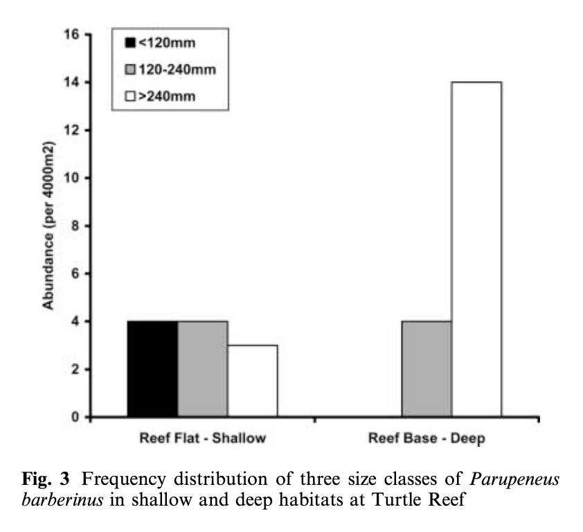
Lukoschek and McCormick’s (2001) study investigating the spatial distribution of a benthic fish species’ foraging behavior is a great example of combining data on behavior, habitat, and morphology.  They collected data on the diet composition of individual fish categorized into different size classes (small, medium, and large) and what foraging tactics were used in which reef zones and habitat types. The foraging tactics ranged from feeding in the water column to digging (at a range of depths) in the benthic substrate. The results showed that an interesting combination of fish behavior and morphology explained the observed diet composition and spatial distribution patterns. Small fish foraged in shallower water, on smaller prey, and primarily employed the water column and shallow digging tactics. In contrast, large fish foraged in deep water, on larger prey, and primarily fed by digging deeper into the seafloor (Figure 1). This pattern is explained by both morphology and behavior. Morphologically, the size of the feeding apparatus (mouth gape size) affects the size of the prey that a fish can feed on. The gape of the small fish is not large enough to eat the larger prey that large fish are able to consume. Behaviorally, predation risk also affects habitat selection and tactic use. Small fish are at higher risk of being predated on, so they remain in shallow areas where they are more protected from predators and they don’t dig as deep to forage because they need to be able to keep an eye out for predators. Interestingly, while they found a relationship between the morphology of the fish and habitat use, they did not find an association between specific feeding tactics and habitat types.

Figure 1. Figure from Lukoschek and McCormick (2001) showing that small fish (black bar) were found in shallow habitat while large fish (white bar) were found in deep habitat.

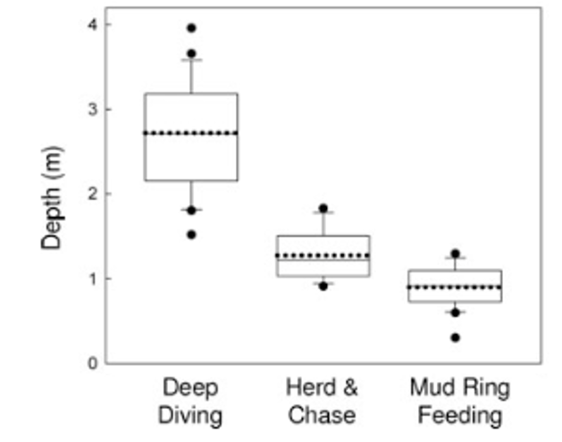
Conversely, Torres and Read (2009) did find associations between theforaging tactics of bottlenose dolphins in Florida Bay, FL and habitat type. Dolphins in this bay employ three foraging tactics: herd and chase, mud ring feeding, and deep diving. Observations of the foraging tactics were linked to habitat characteristics and individual dolphins. The study found that these tactics are spatially structured by depth (Figure 2), with deep diving occurring in deep water whereas mud ring feeding occurrs in shallower water. They also found evidence of individual specialization! Individuals that were observed deep diving were not observed mud ring feeding and vice-versa. Furthermore, they found that individuals were found in the habitat type associated with their preferred tactic regardless of whether they were foraging or not. This result indicates that individual dolphins in this bay have a foraging tactic they prefer and tend to stay in the corresponding habitat type. These findings are really intriguing and raise interesting questions regarding how these tactics and specializations are developed or learned. These are questions that I am also interested in asking as part of my thesis.

Figure 2. Figure from Torres and Read (2009) showing that deep diving is associated with deeper habitat while mud ring feeding is associated with shallow habitat.

Both of these studies are cool examples that, combined, exemplify questions I am interested in examining using our study population of Pacific Coast Feeding Group (PCFG) gray whales. Like both studies, I am interested in assessing how specific foraging tactics are associated with habitat types. Our hypothesis is that different prey types live in different habitat types, so each tactic corresponds to the best way to feed on that prey type in that habitat. While predation risk doesn’t have as much of an effect on foraging gray whales as it does on small benthic fish, I do wonder how disturbance from boats could similarly affect tactic preference and spatial distribution. I am also curious to see if depth has an effect on tactic choice by using the morphology data from our drone-based photogrammetry. Given that these whales forage in water that is sometimes as deep as they are long, it stands to reason that maneuverability would affect tactic use. As described in a previous blog, I’m also looking for evidence of individual specialization. It will be fascinating to see how foraging preference relates to space use, habitat preference, and morphology.

These studies demonstrate the complexity involved in studying a population’s relationship to its habitat. Such research involves considering the morphology and physiology of the animals, their social, individual, foraging, and predator-prey behaviors, and the relationship between their prey and the habitat. It’s a bit daunting but mostly really exciting because better understanding each puzzle piece improves our ability to estimate how these animals will react to changing environmental conditions.

While I don’t have any answers to these questions yet, I will be working with a National Science Foundation Research Experience for Undergraduates intern this summer to develop a habitat map of our study area that will be used in this analysis and potentially answer some preliminary questions about PCFG gray whale habitat use patterns. So, stay tuned to hear more about our work this summer!

References

Lukoschek, V., & McCormick, M. (2001). Ontogeny of diet changes in a tropical benthic carnivorous fish, Parupeneus barberinus (Mullidae): Relationship between foraging behaviour, habitat use, jaw size, and prey selection. Marine Biology, 138(6), 1099–1113. https://doi.org/10.1007/s002270000530

Torres, L. G., & Read, A. J. (2009). Where to catch a fish? The influence of foraging tactics on the ecology of bottlenose dolphins ( Tursiops truncatus ) in Florida Bay, Florida. Marine Mammal Science, 25(4), 797–815. https://doi.org/10.1111/j.1748-7692.2009.00297.x

Connecting Research Questions

Clara Bird, Masters Student, OSU Department of Fisheries and Wildlife, Geospatial Ecology of Marine Megafauna Lab

The field season can be quite a hectic time of year. Between long days out on the water, trouble-shooting technology issues, organizing/processing the data as it comes in, and keeping up with our other projects/responsibilities, it can be quite overwhelming and exhausting.

But despite all of that, it’s an incredible and exciting time of year. Outside of the field season, we spend most of our time staring at our computers analyzing the data that we spend a relatively short amount of time collecting. When going through that process it can be easy to lose sight of why we do what we do, and to feel disconnected from the species we are studying. Oftentimes the analysis problems we encounter involve more hours of digging through coding discussion boards than learning about the animals themselves. So, as busy as it is, I find that the field season can be pretty inspiring. I have recently been looking through our most recent drone footage of gray whales and feeling renewed excitement for my thesis.

At the moment, my thesis has four central questions: (1) Are there associations between habitat type and gray whale foraging tactic? (2) Is there evidence of individualization? (3) What is the relationship between behavior and body condition? (4) Do we see evidence of learning in the behavior of mom and calf pairs? As I’ve been organizing my thoughts, what’s become quite clear is how interconnected these questions are. So, I thought I’d take this blog to describe the potential relationships.

Let’s start with the first question: are there associations between habitat types and gray whale foraging tactics? This question is central because it relates foraging behavior to habitat, which is ultimately associated with prey. This relationship is the foundation of all other questions involving foraging tactics because food is necessary for the whales to have the energy and nutrients they need to survive. It’s reasonable to think that the whales are flexible and use different foraging tactics to eat different prey that live in different habitats. But, if different prey types have different nutritional value (this is something that Lisa is studying right now; check out the COZI project to learn more), then not all whales may be getting the same nutrients.

The next question relates to the first question but is not necessarily dependent on it. It’s the question of individualization, a topic Lisa also explored in a past blog. Within our Oregon field sites we have documented a variety of gray whale foraging tactics (Torres et al. 2018; Video 1) but we do not know if all gray whales use all the tactics or if different individuals only use certain tactics. While I think it’s unlikely that one whale only uses one tactic all the time, I think we could see an individual use one tactic more often than the others. I reason that there could be two reasons for this pattern. First, it could be a response to resource availability; certain tactics are more efficient than others, this could be because the tactic involves capturing the more nutritious prey or because the behavior is less energetically demanding. Second, foraging tactics are socially learned as calves from their mothers, and hence individuals use those learned tactics more frequently. This pattern of maternally inherited foraging tactics has been documented in other marine mammals (Mann and Sargeant 2009; Estes et al. 2003). These questions between foraging tactic, habitat and individualization also tie into the remaining two questions.

My third question is about the relationship between behavior and body condition. As I’ve discussed in a previous blog, I am interested in assessing the relative energetic costs and benefits of the different foraging tactics. Is one foraging tactic more cost-effective than another (less energy out per energy in)? Ever since our lab’s cetacean behavioral ecology class, I’ve been thinking about how my work relates to niche partitioning theory (Pianka 1974).This theory states that when there is low prey availability, niche partitioning will increase. Niche partitioning can occur across several different dimensions: for instance, prey type, foraging location, and time of day when active. If gray whales partition across the prey type dimension, then different whales would feed on different kinds of prey. If whales partition resources across the foraging location dimension, individuals would feed in different areas. Lastly, if whales partition resources across the time axis, individuals would feed at different times of day. Using different foraging tactics to feed on different prey would be an example of partitioning across the prey type dimension. If there is a more preferable prey type, then maybe in years of high prey availability, we would see most of the gray whales using the same tactics to feed on the same prey type. However, in years of low prey availability we might expect to see a greater variety of foraging tactics being used. The question then becomes, does any whale end up using the less beneficial foraging tactic? If so, which whales use the less beneficial tactic? Do the same individuals always switch to the less beneficial tactic? Is there a common characteristic among the individuals that switched, like sex, age, size, or reproductive status? Lemos et al. (2020) hypothesized that the decline in body condition observed from 2016 to 2017 might be a carryover effect from low prey availability in 2016. Could it be that the whales that use the less beneficial tactic exhibit poor body condition the following year?

My fourth, and final, question asks if foraging tactics are passed down from moms to their calves. We have some footage of a mom foraging with her calf nearby, and occasionally it looks like the calf could be copying its mother. Reviewing this footage spiked my interest in seeing if there are similarities between the behavior tactics used by moms and those used by their calves after they have been weaned. While this question clearly relates to the question of individualization, it is also related to body condition: what if the foraging tactics used by the mom is influenced by her body condition at the time?

I hope to answer some of these fascinating questions using the data we have collected during our long field days over the past 6 years. In all likelihood, the story that comes together during my thesis research will be different from what I envision now and will likely lead to more questions. That being said, I’m excited to see how the story unfolds and I look forward to sharing the evolving ideas and plot lines with all of you.

References

Estes, J A, M L Riedman, M M Staedler, M T Tinker, and B E Lyon. 2003. “Individual Variation in Prey Selection by Sea Otters: Patterns, Causes and Implications.” Source: Journal of Animal Ecology. Vol. 72.

Mann, Janet, and Brooke Sargeant. 2009. “ Like Mother, like Calf: The Ontogeny of Foraging Traditions in Wild Indian Ocean Bottlenose Dolphins ( Tursiops Sp.) .” In The Biology of Traditions, 236–66. Cambridge University Press. https://doi.org/10.1017/cbo9780511584022.010.

Pianka, Eric R. 1974. “Niche Overlap and Diffuse Competition” 71 (5): 2141–45.

Soledade Lemos, Leila, Jonathan D Burnett, Todd E Chandler, James L Sumich, and Leigh G. Torres. 2020. “Intra‐ and Inter‐annual Variation in Gray Whale Body Condition on a Foraging Ground.” Ecosphere 11 (4). https://doi.org/10.1002/ecs2.3094.

Torres, Leigh G., Sharon L. Nieukirk, Leila Lemos, and Todd E. Chandler. 2018. “Drone up! Quantifying Whale Behavior from a New Perspective Improves Observational Capacity.” Frontiers in Marine Science 5 (SEP). https://doi.org/10.3389/fmars.2018.00319.

Whale blow: good for more than spotting whales

Clara Bird, Masters Student, OSU Department of Fisheries and Wildlife, Geospatial Ecology of Marine Megafauna Lab

Whale blow, the puff of air mixed with moisture that a whale releases when it comes to the surface, is a famously thrilling indicator of the presence of a whale. From shore, spotting whale blow brings the excitement of knowing that there are whales nearby. During boat-based field work, seeing or hearing blow brings the rush of adrenaline meaning that it’s game time. Whale blow can also be used to identify different species of whales, for example gray whale blow is heart shaped (Figure 1). However, whale blow can be used for more than just spotting and identifying whales. We can use the time between blows to study energetics.

Figure 1. Gray whale blow is often heart shaped (when there is very little wind). Source: https://www.lajollalight.com/sdljl-natural-la-jolla-winter-wildlife-2015jan08-story.html

A blow interval is the time between consecutive blows when a whale is at the surface (Stelle, Megill, and Kinzel 2008). These are also known as short breath holds, whereas long breath holds are times between surfacings (Sumich 1983).  Sumich (1983) hypothesized that short breath holds lead to efficient rates of oxygen use. The body uses oxygen to create energy, so “efficient rate of oxygen use” means that longer breath holds do not use much more oxygen and subsequently do not produce more energy.  Surfacings, during which short blow intervals occur, are often thought of as recovery periods for whales. Think of it this way, when you sprint, immediately afterwards you typically need to take a break to just breathe and recover.

We hypothesize that we can use blow intervals as a measure of how strenuous an activity is; shorter blow intervals may indicate that an activity is more energetically demanding (Wursig, Wells, and Croll 1986). Let’s go back to the sprinting analogy and compare the energetic demands of walking and running. Imagine I asked you to walk for five minutes, stop and measure the time between each breath, and then run for five minutes and do the same; after running, you would likely breathe more heavily and take more breaths with less time between them. This result indicates that running is more demanding, which we already know because we can do other experiments with humans to study metabolic rate and related metrics. In the case of gray whales, we cannot do experiments in the same way, but we can use the same analogy. Several studies have examined how blow intervals differ between travelling and foraging.

Wursig, Wells, and Croll (1986) measured blow interval, surfacing time, and estimated dive depth and duration of gray whales in Alaska from a boat during the foraging season. They found that blow intervals were shorter during feeding. They also found that the number of blows per surfacing increased with increasing depth. Overall these findings suggest that during the foraging season, feeding is more strenuous than other behaviors and that deeper dives may be more physiologically stressful.

Stelle, Megill, and Kinzel (2008) studied gray whales foraging off of British Columbia, Canada. They found shorter blow intervals during foraging, intermediate blow intervals during searching, and longer blow intervals during travelling. Interestingly, within feeding behaviors, they found a difference between whales feeding on mysids (krill-like animals that swim in the water column) and whales feeding benthically on amphipods. They found that whales feeding on mysids made more frequent but shorter dives with short blow intervals at surface, while whales feeding benthically had longer dives with longer blow intervals. They hypothesized that this difference in surfacing pattern is because mysids might scatter when disturbed, so gray whales surface more often to allow the mysids swarm to reform. These studies inspired me to start investigating these same questions with my drone video data.

As I review the drone footage and code the behaviors I also mark the time of each blow. I’ve done some initial video coding and using this data I have started to look into differences in blow intervals. As it turns out, we see a similar difference in blow interval relative to behavior state in our data: whales that are foraging have shorter blow intervals than when traveling (Figure 2). It is encouraging to see that our data shows similar patterns.

Figure 2. Boxplot of mean blow interval per sighting of foraging whales and travelling whales.

Next, I would like to examine how blow intervals differ between foraging tactics. A significant part of my thesis is dedicated to studying specific foraging tactics. The perspective from the drone allows us to identify behaviors in greater detail than studies from shore or boat (Torres et al. 2018), allowing us to dig into the differences between the different foraging behaviors. The purpose of foraging is to gain energy. However, this gain is a net gain. To understand the different energetic “values” of each tactic we need to understand the cost of each behavior, i.e. how much energy is required to perform the behavior. Given previous studies, maybe blow intervals could help us measure this cost or at least compare the energetic demands of the behaviors relative to each other. Furthermore, because different behaviors are likely associated with different prey types (Dunham and Duffus 2001), we also need to understand the different energetic gains of each prey type (this is something that Lisa is studying right now, check out the COZI project to learn more). By understanding both of these components – the gains and costs – we can understand the energetic tradeoffs of the different foraging tactics.

Another interesting component to this energetic balance is a whale’s health and body condition. If a whale is in poor health, can it afford the energetic costs of certain behaviors? If whales in poor body condition engage in different behavior patterns than whales in good body condition, are these patterns explained by the energetic costs of the different foraging behaviors? All together this line of investigation is leading to an understanding of why a whale may choose to use different foraging behaviors in different situations. We may never get the full picture; however, I find it really exciting that something as simple and non-invasive as measuring the time between breaths can contribute such a valuable data stream to this project.

References

Dunham, Jason S., and David A. Duffus. 2001. “Foraging Patterns of Gray Whales in Central Clayoquot Sound, British Columbia, Canada.” Marine Ecology Progress Series 223 (November): 299–310. https://doi.org/10.3354/meps223299.

Stelle, Lei Lani, William M. Megill, and Michelle R. Kinzel. 2008. “Activity Budget and Diving Behavior of Gray Whales (Eschrichtius Robustus) in Feeding Grounds off Coastal British Columbia.” Marine Mammal Science 24 (3): 462–78. https://doi.org/10.1111/j.1748-7692.2008.00205.x.

Sumich, James L. 1983. “Swimming Velocities, Breathing Patterns, and Estimated Costs of Locomotion in Migrating Gray Whales, Eschrichtius Robustus.” Canadian Journal of Zoology 61 (3): 647–52. https://doi.org/10.1139/z83-086.

Torres, Leigh G., Sharon L. Nieukirk, Leila Lemos, and Todd E. Chandler. 2018. “Drone up! Quantifying Whale Behavior from a New Perspective Improves Observational Capacity.” Frontiers in Marine Science 5 (SEP). https://doi.org/10.3389/fmars.2018.00319.

Wursig, B., R. S. Wells, and D. A. Croll. 1986. “Behavior of Gray Whales Summering near St. Lawrence Island, Bering Sea.” Canadian Journal of Zoology 64 (3): 611–21. https://doi.org/10.1139/z86-091.

Are Oregon gulls trash birds?

By Stephanie Loredo, MSc student

“Violent” and “greedy” are words often used to describe gulls in populous areas where food or trash are readily available.  Humans are used to seeing gulls in parking lots, parks, and plazas eating left over crumbs. Many people have even experienced menacing gulls ripping food away from their hands. Anecdotes like these have caused people to have negative perceptions of gulls. But could the repulsive attitude towards these birds be changed with evidence that not all gulls are the same? Well, Oregon may be home to an odd bunch.

Last year, the Seabird Oceanography Lab in conjunction with the GEMM Lab began putting GPS trackers on western gulls (Laurus occidentalis) off the Oregon Coast. One of the goals was to determine where gulls scavenge for food while raising chicks: at sea or on land in association with humans. We were particularly interested to see if western gulls in Oregon would behave similarly to western gulls in California, some of which make trips to the nearest landfill during the breeding season to bring not only food but also potentially harmful pathogens back to the colony.

During the 2015 breeding season, 10 commercially brand ‘i-gotU’ GPS data loggers were placed on gulls from ‘Cleft-in-the-Rock’ colony in Yachats, Oregon. The tags provided GPS locations at intervals of two minutes that determined the general habitat use areas (marine vs. terrestrial). After a two-week period, we were able to recapture six birds, remove tags, and download the data.   We found that these western gulls stayed close to the colony and foraged in nearby intertidal and marine zones (Figure 1). Birds showed high site faithfulness by visiting the same foraging spots away from colony. It was interesting to see that inland habitat use did not extend past 1.3 miles from shore and the only waste facility within such boundaries did not attract any birds (Figure 1). Tagged birds never crossed the 101 Highway, but rather occurred at beaches in state parks such as Neptune and Yachats Ocean Road.

Figure 1. Tracks from 6 western gulls, each color representing a unique bird, from the Cleft-in-the-Rock colony carrying micro-GPS units.

While it is hard to determine whether gulls avoided anthropogenic sources of food at the beach, preliminary analysis shows a high percentage of time spent in marine and intertidal habitat zones by half of the individuals (Figure 2). At a first glance, this is not as much as it seemed on the tracking map (Figure 1), but it nonetheless confirms that these gulls seek food in natural areas. Moreover, time spent at the colony is represented as time spent on coastal habitat on the graph, and thus “coastal” foraging values are over represented. To get a more exact estimate of coastal habitat use, future analysis will have to exclude colony locations and distinguish foraging versus resting behaviors.

Figure 2. Bar plot of the percentage of time spent in three distinct habitats for each gull carrying a GPS unit. The three-letter code represents the unique Bird ID.

‘Cleft-in-the-Rock’ is unique and its surroundings may explain why there was high foraging in intertidal and marine zones rather than within city limits. (The Cleft colony can also be tricky to get to, with a close eye on the tide at all times – See video below).  The colony site is close to the Cape Perpetua Scenic Area and surrounded by recently established conservation zones: the Cape Perpetua Marine Reserve Area, Marine Protected Area, and Seabird Protected Area (Figure 1).  Each of these areas has different regulatory rules on what is allowed to take, which you can read about here. The implication of these protected areas in place means there is more food for wildlife!  Moreover, the city of Yachats has a small population of 703 inhabitants (based on 2013 U.S Census Bureau). The small population allows the city to be relatively clean, and the waste facility is not spewing rotten odors into the air like in many big cities such as Santa Cruz (population of 62,864) where our collaborative gull study takes place. Thus, in Yachats, there is more limited odor or visual incentive to attract birds to landfills.

Field crew descends headland slope to reach ‘Cleft-in-the-Rock’ gull island in Yachats, OR (colony can be seen in distance across the water). The team must wear wetsuits and carry equipment in dry bags for protection during water crossing.

In order to determine whether gull habitat use in Yachats is a trend for all western gulls in Oregon, we need to track birds at more sites and for a longer time. That is why during the breeding season of 2016, we will be placing 30 new tags on gulls and include a new colony into the study, ‘Hunters Island’. The new colony is situated near the Pistol River, between Gold Beach and Brookings in southern Oregon, and it is part of the Oregon Islands Wildlife Refuge.

We will have 10 ‘i-gotU’ tags (Figure 3) and 20 CATS tags (Figure 4), the latter are solar powered and can collect data for several weeks, months, and hopefully even years! These tags do not need to be retrieved for data download; rather data can be accessed remotely, providing minimal disturbance to the gulls and colony. With long-term data, we can explore further into the important feeding areas for western gulls, examine rates of foraging in different habitats, and determine how extensive intertidal and marine foraging is throughout the year.

Figure 3. Taping an i-gotU tag for temporary attachment on the tail feathers of a gull.


Figure 4. Rehearsing the placement and harness attachment of a CATS tag which must be secured on the bird‘s back, looping around the wings and hips.

We are excited to kick start our field season in the next couple of weeks and see how well the new tags work. We know that some questions will be solved and many new questions will arise; and we cannot wait to start this gull-filled adventure!

References

Osterback, A.M., Frechette, D., Hayes, S., Shaffer, S., & Moore, J. (2015). Long-term shifts in anthropogenic subsidies to gulls and implications for an imperiled fish. Biological Conservation191: 606–613.

Scratching the Surface

By Dr. Leigh Torres, Assistant Professor, Oregon State University, Geospatial Ecology of Marine Megafauna Lab

I have been reminded of a lesson I learned long ago: Never turn your back on the sea – it’s always changing.

The blue whales weren’t where they were last time. I wrongly assumed oceanographic patterns would be similar to our last time out in 2014 and that the whales would be in the same area. But the ocean is dynamic – ever changing. I knew this. And I know it better now.

Below (Fig. 1) are two satellite images of sea surface temperature (SST) within the South Taranaki Bight and west coast region of New Zealand that we surveyed in Jan-Feb 2014 and again recently during Jan-Feb 2016. The plot on the left describes ocean surface conditions in 2014 and illustrates how SST primarily ranged between 15 and 18 ⁰C. By comparison, the panel on the right depicts the sea surface conditions we just encountered during the 2016 field season, and a huge difference is apparent: this year SST ranged between 18 and 23 ⁰C, barely overlapping with the 2014 field season conditions.

Figure 1. A comparison of satellite images of sea surface temperature (SST) in the South Taranaki Bight region of New Zealand between late January 2014 and early February 2016. The white circles on each image denote where the majority of blue whales were encountered during each field season.

While whales can live in a wide range of water temperatures, their prey is much pickier. Krill, tiny zooplankton that blue whales seek and devour in large quantities, tend to aggregate in pockets of nutrient-rich, cool water in this region of New Zealand. During the 2014 field season, we encountered most blue whales in an area where SST was about 15 ⁰C (within the white circle in the left panel of Fig. 1). This year, there was no cool water anywhere and we mainly found the whales off the west coast of Kahurangi shoals in about 21 ⁰C water (within the white circle in the right panel of Fig. 1. NB: the cooler water in the Cook Strait in the southeast region of the right panel is a different water mass than preferred by blue whales and does not contain their prey.)

The hot water we found this year across the survey region can likely be attributed, at least in part, to the El Niño conditions that are occurring across the Pacific Ocean currently. El Niño has brought unusually settled conditions to New Zealand this summer, which means relatively few high wind events that normally churn up the ocean and mix the cool, nutrient rich deep water with the hot surface layer water. These are ideal conditions for Kiwi sun-bathers, but the ocean remains highly stratified with a stable layer of hot water on top. However, this stratification does not necessarily mean the ocean is un-productive – it only means that the SST satellite images are virtually useless for helping us to find whales this year.

Although SST data can be informative about ocean conditions, it only reflects what is happening in the thin, top slice of the ocean. Sub-surface conditions can be very different. Ocean conditions during our two survey periods in 2014 and 2016 could be more similar when compared underwater than when viewed from above. This is why sub-surface sensors and data collection is critical to marine studies. Ocean conditions in 2014 and 2016 could both potentially provide good habitat for the whales. In fact, where and when we encountered whales during both 2014 and 2016 we also detected high densities of krill through hydro-acoustics (Fig. 2). However, in 2014 we observed many surface swarms of krill that we rarely saw this recent field season, which could be due to elevated SST. But, we did capture cool drone footage this year of a brief sub-surface foraging event:

An overhead look of a blue whale foraging event as the animal approaches the surface. Note how the distended ventral (throat) grooves of the buccal cavity (mouth) are visible. This is a big gulp of prey (krill) and water. The video was captured using a DJI Phantom 3 drone in the South Taranaki Bight of New Zealand in on February 2, 2016 under a research permit from the New Zealand Department of Conservation (DOC) permit # 45780-MAR issued to Oregon State University.

Figure 2. An echo-sounder image of dense krill patches at 50-80 m depth captured through hydroacoustics in the South Taranaki Bight region of New Zealand.

Below are SST anomaly plots of January 2014 and January 2016 (Fig. 3). These anomaly plots show how different the SST was compared to the long-term average SST across the New Zealand region. As you can see, in 2014 (left panel) SST conditions in our study area were ~1 ⁰C below average, while in 2016 (right panel) SST conditions were ~1 ⁰C above average. So, what are normal conditions? What can we expect next year when we come back to survey again for blue whales across this region? These are challenging questions and illustrate why marine ecology studies like this one must be conducted over many years. One year is just a snap shot in the lifetime of the oceans.

Figure 3. Comparison of sea surface temperature (SST) anomaly plots of the New Zealand region between January 2014 (left) and January 2016 (right). The white box in both plots denotes the general location of our blue whale study region. (Apologies for the different formats of these plots - the underlying data is directly comparable.)
Figure 3. Comparison of sea surface temperature (SST) anomaly plots of the New Zealand region between January 2014 (left) and January 2016 (right). The white box in both plots denotes the general location of our blue whale study region. (Apologies for the different formats of these plots – the underlying data is directly comparable.)

Like all marine megafauna, blue whales move far and fast to adjust their distribution patterns according to ocean conditions. So, I can’t tell you what the ocean will be like in January 2017 or where the whales will be, but as we continue to study this marine ecosystem and its inhabitants our understanding of ocean patterns and whale ecology will improve. With every year of new data we will be able to better predict ocean and blue whale distribution patterns, providing managers with the tools they need to protect our marine environment. For now, we are just beginning to scratch the (sea) surface.