Taking a breather

Allison Dawn, new GEMM Lab Master’s student, OSU Department of Fisheries, Wildlife and Conservation Sciences, Geospatial Ecology of Marine Megafauna Lab

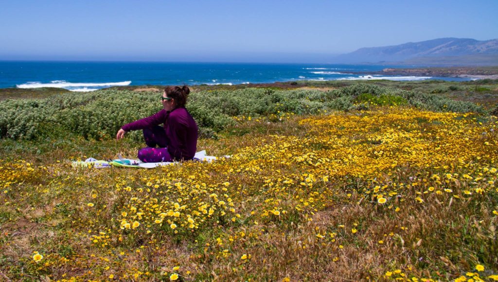
While standing at the Stone Shelter at the Saint Perpetua Overlook in 2016, I took in the beauty of one of the many scenic gems along the Pacific Coast Highway. Despite being an East Coast native, I felt an unmistakable draw to Oregon. Everything I saw during that morning’s hike, from the misty fog that enshrouded evergreens and the ocean with mystery, to the giant banana slugs, felt at once foreign and a place I could call home. Out of all the places I visited along that Pacific Coast road trip, Oregon left the biggest impression on me.

Figure 1. View from the Stone Shelter at the Cape Perpetua Overlook, Yachats, OR. June 2016.

For my undergraduate thesis, which I recently defended in May 2021, I researched blue whale surface interval behavior. Surface interval events for oxygen replenishment and rest are a vital part of baleen whale feeding ecology, as it provides a recovery period before they perform their next foraging dive (Hazen et al., 2015; Roos et al., 2016). Despite spending so much time studying the importance of resting periods for mammals, that 2016 road trip was my last true extended resting period/vacation until, several years later in 2021, I took another road trip. This time it was across the country to move to the place that had enraptured me.

Now that I am settled in Corvallis, I have reflected on my journey to grad school and my recent road trip; both prepared me for a challenging and exciting new chapter as an incoming MSc student within the Marine Mammal Institute (MMI).

Part 1: Journey to Grad School

When I took that photo at the Cape Perpetua Overlook in 2016, I had just finished the first two semesters of my undergraduate degree at UNC Chapel Hill. As a first-generation, non-traditional student those were intense semesters as I made the transition from a working professional to full-time undergrad.

By the end of my freshman year I was debating exactly what to declare as my major, when one of my marine science TA’s, Colleen, (who is now Dr. Bove!), advised that I “collect experiences, not degrees.” I wrote this advice down in my day planner and have never forgotten it. Of course, obtaining a degree is important, but it is the experiences you have that help lead you in the right direction.

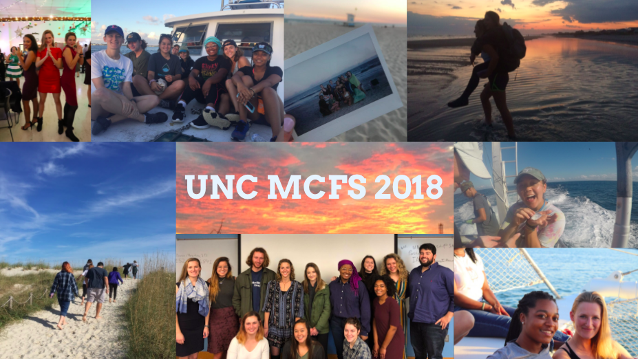
That advice was one of the many reasons I decided to participate in the Morehead City Field Site program, where UNC undergraduates spend a semester at the coast, living on the Duke Marine Lab’s campus in Beaufort, NC. During that semester, students take classes to fulfill a marine science minor while participating in hands-on research, including an honors thesis project. The experience of designing, carrying out, and defending my own project affirmed that graduate school in the marine sciences was right for me. As I move into my first graduate TA position this fall, I hope to pay forward that encouragement to other undergraduates who are making decisions about their own future path.

Figure 2. Final slide from my honors thesis defense. UNC undergraduates, and now fellow alumni, who participated in the Morehead City Field Site program in Fall 2018.

Part 2: Taking a Breather

Like the GEMM Lab’s other new master’s student Miranda, my road trip covered approximately 2,900 miles. I was solo for much of the drive, which meant there was no one to argue when I decided to binge listen to podcasts. My new favorite is How To Save A Planet, hosted by marine biologist Dr. Ayana Elizabeth Johnson and Alex Blumberg. At the end of each episode they provide a call to action & resources for listeners – I highly recommend this show to anyone interested in what you can do right now about climate change.

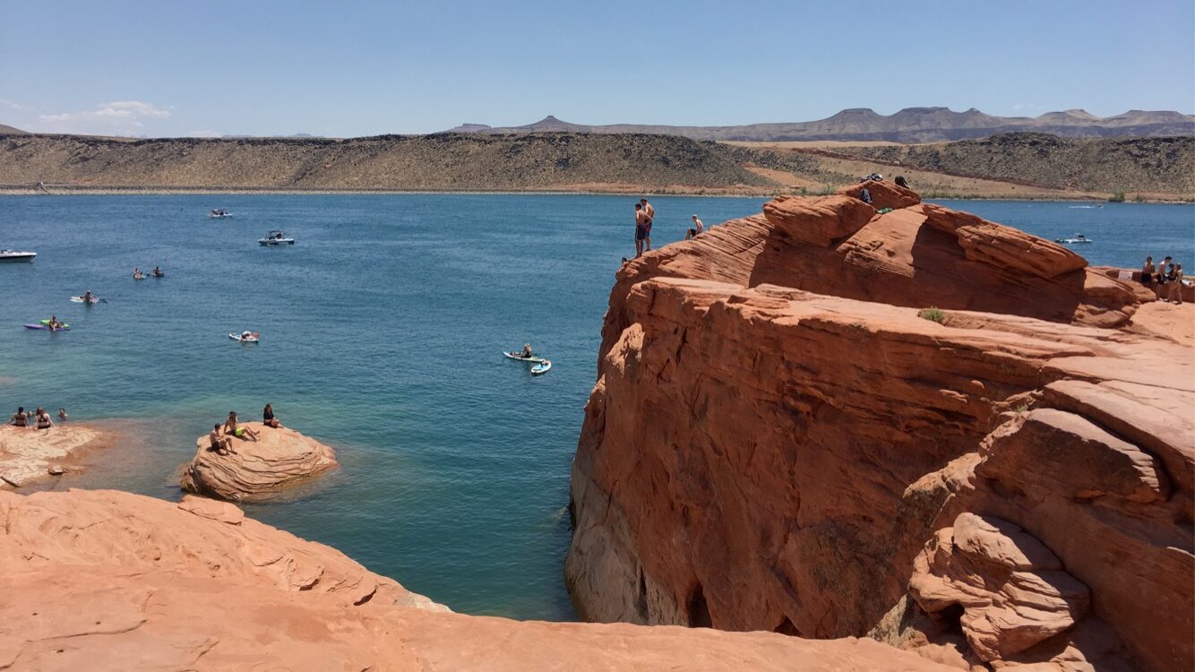
Along my trip I took a stop in Utah to visit my parents. I had never been to a desert basin before and engaged in many desert-related activities: visiting Zion National Park, hiking in 116-degree heat, and facing my fear of heights via cliff jumping.

Figure 3. Sandstone Rocks at Sand Hollow National Park, Hurricane, Utah. June 2021.

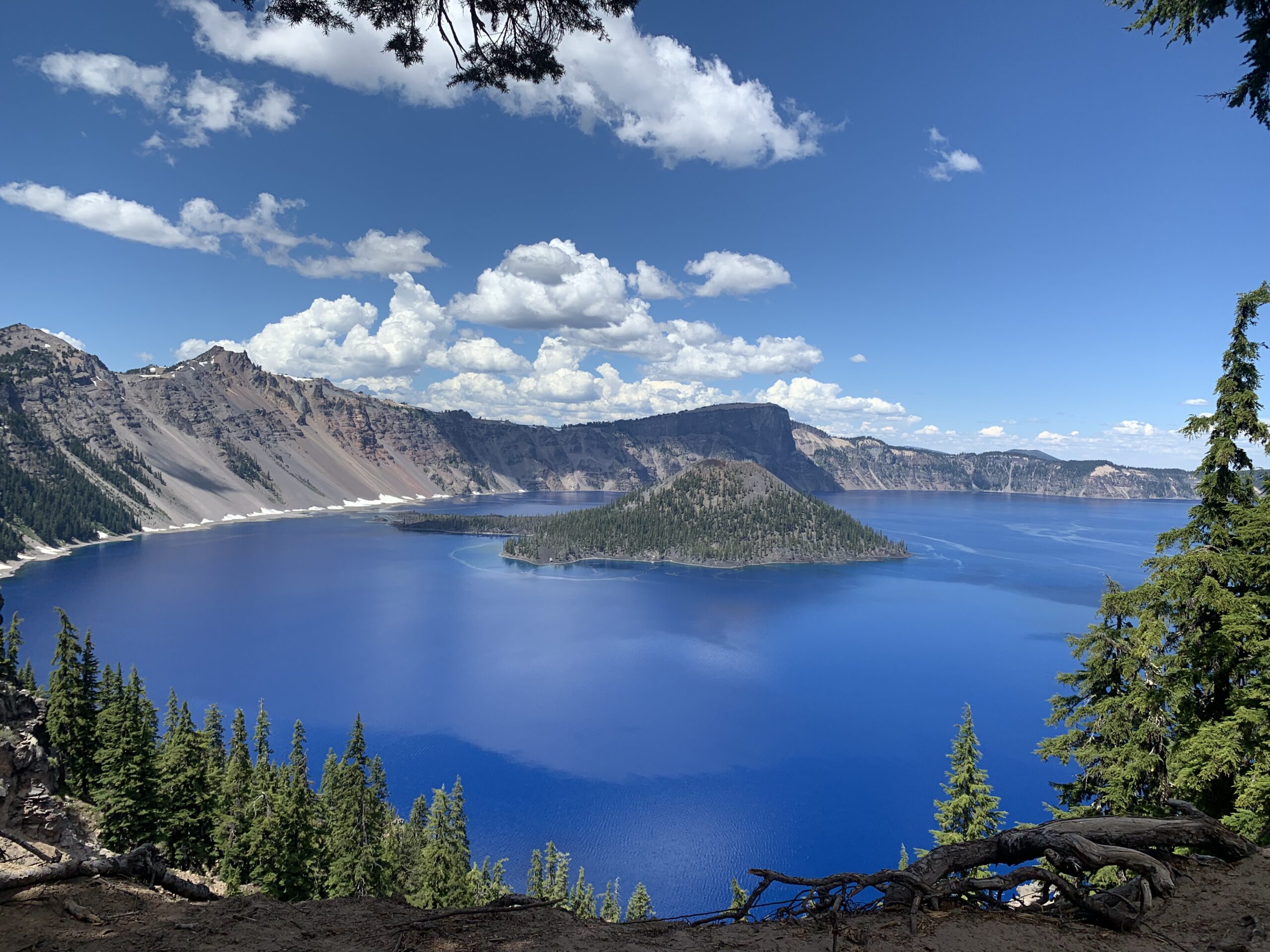
 My parents wanted to help me settle into my new home, as parents do, so we drove the rest of the way to Oregon together. As this would be their first visit to the state, we strategically planned a trip to Crater Lake as our final scenic stop before heading into Corvallis.

Figure 4. Wizard Island in Crater Lake National Park, Klamath County, OR. June 2021.

This time off was filled with adventure, yet was restorative, and reminded me the importance of taking a break. I feel ready and refreshed for an intense summer of field work.

Part 3: Rested and Ready

Despite accumulating skills to do research in the field over the years, I have yet to do marine mammal field work (or even see a whale in person for that matter.) My mammal research experience included analyzing drone imagery, behind a computer, that had already been captured. As you can imagine, I am extremely excited to join the Port Orford team as part of the TOPAZ/JASPER projects this summer, collecting ecological data on gray whales and their prey. I will be learning the ropes from Lisa Hildebrand and soaking up as much information as possible as I will be taking over as lead for this project next year.

It will take some time before my master’s thesis is fully developed, but it will likely focus on assessing the environmental factors that influence gray whale zooplankton prey availability, and the subsequent impacts on whale movements and health. For five years, the Port Orford project has conducted GoPro drops at 12 sampling stations to collect data on zooplankton relative abundance.

Figures 5 & 6. GEMM GoPro drop stick assembly and footage demonstrating mysid data collection. July 2021.

Paired with this GoPro is a Time-Depth Recorder (TDR) that provides temperature and depth data. The 2021 addition to this GoPro system is a new dissolved oxygen (DO) sensor the GEMM Lab has just acquired. This new piece of equipment will add to the set of parameters we can analyze to describe what and how oceanographic factors drive prey variability and gray whale presence in our study site.My first task as a GEMM Lab student is to get to know this DO sensor, figure out how it works, set it up, test it, attach it to the GoPro device, and prepare it for data collection during the upcoming Port Orford project starting in 1 week!

Figure 7. The GEMM lab’s new RBR solo3 getting ready for Port Orford. July 2021.

Dissolved oxygen plays a vital role in the ocean; however, climate change and increased nutrient loading has caused the ocean to undergo deoxygenation. According to the IUCN’s 2019 Issues Brief, these factors have resulted in an oxygen decline of 2% since the middle of the 20th century, with most of this loss occurring within the first 1000 meters of the ocean. Two percent may not seem like much, but many species have a narrow oxygen threshold and, like pH changes in coral reef systems, even slight changes in DO can have an impact. Additionally, the first 1000 meters of the ocean contains the greatest amount of species richness and biodiversity.

Previous research done in a variety of systems (i.e., estuarine, marine, and freshwater lakes) shows that dissolved oxygen concentrations can have an impact on predator-prey interactions, where low dissolved oxygen results in decreased predation (Abrahams et al., 2007; Breitburg et al., 1997; Domenici et al., 2007; Kramer et al., 1987); and changes in DO also change prey vertical distributions (Decker et al., 2004). In Port Orford, we are interested in understanding the interplay of factors driving zooplankton community distribution and abundance while investigating the trophic interaction between gray whales and their prey.

I have spent some time with our new DO sensor and am looking forward to its first deployments in Port Orford! Stay tuned for updates from the field!

References

Abrahams, M. V., Mangel, M., & Hedges, K. (2007). Predator–prey interactions and changing environments: who benefits?. Philosophical Transactions of the Royal Society B: Biological Sciences, 362(1487), 2095-2104.

Breitburg, D. L., Loher, T., Pacey, C. A., & Gerstein, A. (1997). Varying effects of low dissolved oxygen on trophic interactions in an estuarine food web. Ecological Monographs, 67(4), 489-507.

​​Decker, M. B., Breitburg, D. L., & Purcell, J. E. (2004). Effects of low dissolved oxygen on zooplankton predation by the ctenophore Mnemiopsis leidyi. Marine Ecology Progress Series, 280, 163-172.

Domenici, P., Claireaux, G., & McKenzie, D. J. (2007). Environmental constraints upon locomotion and predator–prey interactions in aquatic organisms: an introduction.

Hazen, E. L., Friedlaender, A. S., & Goldbogen, J. A. (2015). Blue whales (Balaenoptera musculus) optimize foraging efficiency by balancing oxygen use and energy gain as a function of prey density. Science Advances, 1(9), e1500469.

Kramer, D. L. (1987). Dissolved oxygen and fish behavior. Environmental biology of fishes, 18(2), 81-92.

Roos, M. M., Wu, G. M., & Miller, P. J. (2016). The significance of respiration timing in the energetics estimates of free-ranging killer whales (Orcinus orca). Journal of Experimental Biology, 219(13), 2066-2077.

“Do Dolphins Get Hives?”: The Skinny on Allergies in Cetaceans

By: Alexa Kownacki, Ph.D. Student, OSU Department of Fisheries and Wildlife, Geospatial Ecology of Marine Megafauna Lab 

While sitting on my porch and watching the bees pollinate the blooming spring flowers, I intermittently pause to scratch the hives along my shoulders and chest. In the middle of my many Zoom calls, I mute myself and stop my video because a wave of pollen hits my face and I immediately have to sneeze. With this, I’m reminded: Welcome to prime allergy season in the Northern Hemisphere. As I was scratching my chronic idiopathic urticaria (hives caused by an overactive immune system), I asked myself “Do dolphins get hives?” I had no idea. I know most terrestrial mammals can and do—just yesterday, one of the horses in the nearby pasture was suffering from a flare of hives. But, what about aquatic and marine mammals? 

Springtime flowers blooming on the Central California Coast 2017. (Image Source: A. Kownacki)

As with most research on marine mammal health, knowledge is scare and is frequently limited to studies conducted on captive and stranded animals. Additionally, most of the current theories on allergic reactions in marine mammals are based on studies from terrestrial wildlife and humans. Because nearly all research on histamine pathways centers on terrestrial animals, I wanted to see what information exists the presence of skin allergies in marine mammals.  

Allergic reactions trigger a cascade within the body, beginning with the introduction of a foreign body, which for many people is pollen. The allergen binds to antibodies that are produced to fight potentially harmful substances. Once this allergen binds to different types of cells, including mast cells, chemicals like histamines are released. Histamines cause the production of mucus and constriction of blood vessels, and thus are the reason your eyes water, your nose runs, or you start coughing. 

Basic cartoon of an allergic reaction from exposure to the allergen to the reaction from the animal. (Image Source: Scientific Malaysian)

As you probably can tell just by looking at a marine mammal, they have thicker skin and fewer mucus membranes that humans, due to the fact that they live in the water. However, mast cells or mast cell-like cells have been described in most vertebrate lineages including mammals, birds, reptiles, amphibians, and bony fishes (Hellman et al. 2017, Reite and Evenson 2006). Mast cell-like cells have also been described in an early ancestor of the vertebrates, the tunicate, or sea squirt (Wong et al. 2014). Therefore, allergic-reaction cascades that may present as hives, red and itchy eyes or nose in humans, also exist in marine mammals, but perhaps cause different or less visible symptoms.  

Skin conditions in cetaceans are gathering interest within the marine mammal health community. Even our very own Dawn BarlowDr. Leigh Torres, and Acacia Pepper assessed the skin conditions in New Zealand blue whales in their recent publication. Most visible skin lesions or markings on cetaceans are caused by parasites, shark bits, fungal infections, and fishery or boat interactions (Leone et al. 2019, Sweeney and Ridgway 1985). However, there is very little scientific literature about allergic reactions in marine mammals, let alone cetaceans. That being said, I managed to find a few critical pieces of information supporting the theory that marine mammals do in fact have allergies that can produce dermal reactions similar to hives in humans.  

In one study, three captive bottlenose dolphins developed reddened skin, sloughing, macules, and wheals on their ventral surfaces (Monreal-Pawlowsky et al. 2017). The medical staff first noticed this atopic dermatitis in 2005 and observed the process escalate over the next decade. Small biopsy samples from the affected areas on the three dolphins coincided with the appearance of four pollens in the air within the geographic region: Betula, Pistacia, Celtis, and Fagus (Monreal-Pawlowsky et al. 2017). Topical prednisone treatments were applied to the affected areas at various dosages that slowly resolved the skin irritations. Researchers manufactured an allergy vaccine using a combination of the four pollens in hopes that it would prevent further seasonal outbreaks, but it was unsuccessful. In the coming years, the facility intends to adjust the dosages to create a successful vaccine.  

In the three top images, visible skin irritation including redness, macules, wheals, and sloughing are present. In the image below, the above animal was treated with methylprednisolone and the skin irritation subsides. (Monreal-Pawlowsky et al. 2017)

In addition to the above study, there is an unpublished case of suspected allergic reaction to another pollen that produces a pruritic reaction on the ventral areas of dolphins on a seasonal basis (Vicente Arribes, personal communication). Although there are only a few documented cases of environmentally-triggered allergic reactions that are visible on the dermal layer of cetaceans, I believe this evidence makes the case that some cetaceans suffer from allergies much like us. So, next time you’re enjoying the beautiful blooms and annoyingly scratch your eyes, know that you are not alone. 

Image Source: FurEver Family

Citations: 

Barlow DR, Pepper AL and Torres LG (2019) Skin Deep: An Assessment of New Zealand Blue Whale Skin Condition. Front. Mar. Sci. 6:757.doi: 10.3389/fmars.2019.00757 

Hellman LT, Akula S, Thorpe M and Fu Z (2017) Tracing the Origins of IgE, Mast Cells, and Allergies by Studies of Wild Animals. Front. Immunol. 8:1749. doi: 10.3389/fimmu.2017.01749 

Leone AB, Bonanno Ferraro G, Boitani L, Blasi MF. Skin marks in bottlenose dolphins (Tursiops truncatus) interacting with artisanal fishery in the central Mediterranean Sea. PLoS One. 2019;14(2):e0211767. Published 2019 Feb 5. doi:10.1371/journal.pone.0211767 

Monreal-Pawlowsky T, Fernández-Bellon H, Puigdemont A (2017) Suspected Allergic Reaction in Bottlenose Dolphins (Tursiops truncatus). J Vet Sci Ani Husb 5(1): 108. doi: 10.15744/2348-9790.5.108 

Reite OB, Evensen O. Inflammatory cells of teleostean fish: a review focusing on mast cells/eosinophilic granule cells and rodlet cells. Fish Shellfish Immunol (2006) 20:192–208. doi:10.1016/j.fsi.2005.01.012 

Sweeney, J. C., & Ridgway, S. H. (1975). Common diseases of small cetaceans. J. Am. Vet. Med. Assoc167(7), 533-540. 

Wong GW, Zhuo L, Kimata K, Lam BK, Satoh N, Stevens RL. Ancient originof mast cells. Biochem Biophys Res Commun (2014) 451:314–8. doi:10.1016/j.bbrc.2014.07.124 

Zooming in: A closer look at bottlenose dolphin distribution patterns off of San Diego, CA

By: Alexa Kownacki, Ph.D. Student, OSU Department of Fisheries and Wildlife, Geospatial Ecology of Marine Megafauna Lab

Data analysis is often about parsing down data into manageable subsets. My project, which spans 34 years and six study sites along the California coast, requires significant data wrangling before full analysis. As part of a data analysis trial, I first refined my dataset to only the San Diego survey location. I chose this dataset for its standardization and large sample size; the bulk of my sightings, over 4,000 of the 6,136, are from the San Diego survey site where the transect methods were highly standardized. In the next step, I selected explanatory variable datasets that covered the sighting data at similar spatial and temporal resolutions. This small endeavor in analyzing my data was the first big leap into understanding what questions are feasible in terms of variable selection and analysis methods. I developed four major hypotheses for this San Diego site.

The study species: common bottlenose dolphin (Tursiops truncatus) seen along the California coastline in 2015. Image source: Alexa Kownacki.

Hypotheses:

H1: I predict that bottlenose dolphin sightings along the San Diego transect throughout the years 1981-2015 exhibit clustered distribution patterns as a result of the patchy distributions of both the species’ preferred habitats, as well as the social nature of bottlenose dolphins.

H2: I predict there would be higher densities of bottlenose dolphin at higher latitudes spanning 1981-2015 due to prey distributions shifting northward and less human activities in the northerly sections of the transect.

H3: I predict that during warm (positive) El Niño Southern Oscillation (ENSO) months, the dolphin sightings in San Diego would be distributed more northerly, predominantly with prey aggregations historically shifting northward into cooler waters, due to (secondarily) increasing sea surface temperatures.

H4: I predict that along the San Diego coastline, bottlenose dolphin sightings are clustered within two kilometers of the six major lagoons, with no specific preference for any lagoon, because the murky, nutrient-rich waters in the estuarine environments are ideal for prey protection and known for their higher densities of schooling fishes.

Data Description:

The common bottlenose dolphin (Tursiops truncatus) sighting data spans 1981-2015 with a few gap years. Sightings cover all months, but not in all years sampled. The same transect in San Diego was surveyed in a small, rigid-hulled inflatable boat with approximately a two-kilometer observation area (one kilometer surveyed 90 degrees to starboard and port of the bow).

I wanted to see if there were changes in dolphin distribution by latitude and, if so, whether those changes had a relationship to ENSO cycles and/or distances to lagoons. For ENSO data, I used the NOAA database that provides positive, neutral, and negative indices (1, 0, and -1, respectively) by each month of each year. I matched these ENSO data to my month-date information of dolphin sighting data. Distance from each lagoon was calculated for each sighting.

Figure 1. Map representing the San Diego transect, represented with a light blue line inside of a one-kilometer buffered “sighting zone” in pale yellow. The dark pink shapes are dolphin sightings from 1981-2015, although some are stacked on each other and cannot be differentiated. The lagoons, ranging in size, are color-coded. The transect line runs from the breakwaters of Mission Bay, CA to Oceanside Harbor, CA.

Results: 

H1: True, dolphins are clustered and do not have a uniform distribution across this area. Spatial analysis indicated a less than a 1% likelihood that this clustered pattern could be the result of random chance (Fig. 1, z-score = -127.16, p-value < 0.0001). It is well-known that schooling fishes have a patchy distribution, which could influence the clustered distribution of their dolphin predators. In addition, bottlenose dolphins are highly social and although pods change in composition of individuals, the dolphins do usually transit, feed, and socialize in small groups.

Figure 2. Summary from the Average Nearest Neighbor calculation in ArcMap 10.6 displaying that bottlenose dolphin sightings in San Diego are highly clustered. When the z-score, which corresponds to different colors on the graphic above, is strongly negative (< -2.58), in this case dark blue, it indicates clustering. Because the p-value is very small, in this case, much less than 0.01, these results of clustering are strongly significant.

H2: False, dolphins do not occur at higher densities in the higher latitudes of the San Diego study site. The sightings are more clumped towards the lower latitudes overall (p < 2e-16), possibly due to habitat preference. The sightings are closer to beaches with higher human densities and human-related activities near Mission Bay, CA. It should be noted, that just north of the San Diego transect is the Camp Pendleton Marine Base, which conducts frequent military exercises and could deter animals.

Figure 3. Histogram comparing the latitudes with the frequency of dolphin sightings in San Diego, CA. The x-axis represents the latitudinal difference from the most northern part of the transect to each dolphin sighting. Therefore, a small difference would translate to a sighting being in the northern transect areas whereas large differences would translate to sightings being more southerly. This could be read from left to right as most northern to most southern. The y-axis represents the frequency of which those differences are seen, that is, the number of sightings with that amount of latitudinal difference, or essentially location on the transect line. Therefore, you can see there is a peak in the number of sightings towards the southern part of the transect line.

H3: False, during warm (positive) El Niño Southern Oscillation (ENSO) months, the dolphin sightings in San Diego were more southerly. In colder (negative) ENSO months, the dolphins were more northerly. The differences between sighting latitude and ENSO index was significant (p<0.005). Post-hoc analysis indicates that the north-south distribution of dolphin sightings was different during each ENSO state.

Figure 4. Boxplot visualizing distributions of dolphin sightings latitudinal differences and ENSO index, with -1,0, and 1 representing cold, neutral, and warm years, respectively.

H4: True, dolphins are clustered around particular lagoons. Figure 5 illustrates how dolphin sightings nearest to Lagoon 6 (the San Dieguito Lagoon) are always within 0.03 decimal degrees. Because of how these data are formatted, decimal degrees is the easiest way to measure change in distance (in this case, the difference in latitude). In comparison, dolphins at Lagoon 5 (Los Penasquitos Lagoon) are distributed across distances, with the most sightings further from the lagoon.

Figure 5. Bar plot displaying the different distances from dolphin sighting location to the nearest lagoon in San Diego in decimal degrees. Note: Lagoon 4 is south of the study site and therefore was never the nearest lagoon.

I found a significant difference between distance to nearest lagoon in different ENSO index categories (p < 2.55e-9): there is a significant difference in distance to nearest lagoon between neutral and negative values and positive and neutral years. Therefore, I hypothesize that in neutral ENSO months compared to positive and negative ENSO months, prey distributions are changing. This is one possible hypothesis for the significant difference in lagoon preference based on the monthly ENSO index. Using a violin plot (Fig. 6), it appears that Lagoon 5, Los Penasquitos Lagoon, has the widest variation of sighting distances in all ENSO index conditions. In neutral years, Lagoon 0, the Buena Vista Lagoon has multiple sightings, when in positive and negative years it had either no sightings or a single sighting. The Buena Vista Lagoon is the most northerly lagoon, which may indicate that in neutral ENSO months, dolphin pods are more northerly in their distribution.

Figure 6. Violin plot illustrating the distance from lagoons of dolphin sightings under different ENSO conditions. There are three major groups based on ENSO index: “-1” representing cold years, “0” representing neutral years, and “1” representing warm years. On the x-axis are lagoon IDs and on the y-axis is the distance to the nearest lagoon in decimal degrees. The wider the shapes, the more sightings, therefore Lagoon 6 has many sightings within a very small distance compared to Lagoon 5 where sightings are widely dispersed at greater distances.


Bottlenose dolphins foraging in a small group along the California coast in 2015. Image source: Alexa Kownacki.

Takeaways to science and management: 

Bottlenose dolphins have a clustered distribution which seems to be related to ENSO monthly indices, and likely, their social structures. From these data, neutral ENSO months appear to have something different happening compared to positive and negative months, that is impacting the sighting distributions of bottlenose dolphins off the San Diego coastline. More research needs to be conducted to determine what is different about neutral months and how this may impact this dolphin population. On a finer scale, the six lagoons in San Diego appear to have a spatial relationship with dolphin sightings. These lagoons may provide critical habitat for bottlenose dolphins and/or for their preferred prey either by protecting the animals or by providing nutrients. Different lagoons may have different spans of impact, that is, some lagoons may have wider outflows that create larger nutrient plumes.

Other than the Marine Mammal Protection Act and small protected zones, there are no safeguards in place for these dolphins, whose population hovers around 500 individuals. Therefore, specific coastal areas surrounding lagoons that are more vulnerable to habitat loss, habitat degradation, and/or are more frequented by dolphins, may want greater protection added at a local, state, or federal level. For example, the Batiquitos and San Dieguito Lagoons already contain some Marine Conservation Areas with No-Take Zones within their reach. The city of San Diego and the state of California need better ways to assess the coastlines in their jurisdictions and how protecting the marine, estuarine, and terrestrial environments near and encompassing the coastlines impacts the greater ecosystem.

This dive into my data was an excellent lesson in spatial scaling with regards to parsing down my data to a single study site and in matching my existing data sets to other data that could help answer my hypotheses. Originally, I underestimated the robustness of my data. At first, I hesitated when considering reducing the dolphin sighting data to only include San Diego because I was concerned that I would not be able to do the statistical analyses. However, these concerns were unfounded. My results are strongly significant and provide great insight into my questions about my data. Now, I can further apply these preliminary results and explore both finer and broader scale resolutions, such as using the more precise ENSO index values and finding ways to compare offshore bottlenose dolphin sighting distributions.

Remote Sensing Applications

By Leila Lemos, PhD candidate

Fisheries and Wildlife Department, OSU


I am finally starting my 3rd and last year of my PhD. Just a year left and yet so many things to do. As per department requirements, I still need to take some class credits, but what classes could I take? In this short amount of time it is important to focus on my research project and on what could help me better understand the many branches of the project and what could improve my analyses. Thinking of that, both my advisor (Dr. Leigh G. Torres) and I agreed that it would be useful for me to take a class on remote sensing. So, I could learn more about this field, as well as try to include some remote sensing analyses in my project, such as sea surface temperature (SST) and chlorophyll (i.e., as a productivity indicator) conditions over the years we have collected data on gray whales off the Oregon coast.


Our photogrammetry data indicates that whales gradually increased their body condition over the feeding seasons of 2016 and 2018, while 2017 is different. Whales were still looking skinny in the middle of the season, and we were not collecting many fecal samples up to that point (indicating not much feeding). These findings made us wonder if this was related to delayed seasonal upwelling events and consequently low prey availability. These questions are what motivated me the most to join this class so that we might be able to link environmental correlates with our observations of gray whale body condition.

Figure 01: Skinny body condition state of the gray whale “Pancake” in August 2017.
Source: Leila S. Lemos


If we stop to think about what remote sensing is, we have already been implementing this method in our project since the beginning, as my favorite definition for remote sensing is “the art of collecting information of objects or phenomenon without touching it”. So, yes, the drone is a type of sensor that remotely collects information of objects (in this case, whales).

Figure 02: Drone remotely collecting information of a whale in September 2018. Drone in detail. Collected under NOAA/NMFS permit #16111.
Source: Leila Lemos


However, satellites, all the way up in the space, are also remotely sensing the Earth and its objects and phenomena. Even from thousands of km above Earth, these sensors are capable of generating a great amount of detailed data that is easily and freely accessible (i.e., NASA, NOAA), and can be used for multiple applications in different fields of study. Satellites are also able to collect data from remote areas like the Antarctica and the Arctic, as well as other areas that are not easily reached by humans. One important application of the use of satellite imagery is wildlife monitoring.

For example, satellite data was used to detect variation in the abundance of Weddell seals (Leptonychotes weddellii) in Erebus Bay, Antarctica (LaRue et al., 2011). Because this is a well-studied seal population, the object of this study was to test if satellite imagery could produce reliable abundance estimates. The authors used high-resolution (0.6 m) satellite imagery (from satellites Quick-Bird-2 and WorldView-1) to compare counts from the ground with counts from satellite images in the same locations at the same time. This study demonstrated a reliable methodology for further studies to replicate.

Figure 03: WorldView-1 image (0.6 m resolution) of Weddell seals hauled out east of Inaccessible Island, Erebus Bay, Antarctica.
Source: LaRue et al. (2011).


Satellite imagery was also applied to estimate colony sizes of Adélie penguins in Antarctica (LaRue et al., 2014). High-resolution (0.6 m) satellite imagery combined with spectral analysiswas used to estimate the sizes of the penguin breeding colonies. Ground counts were also used in order to check the reliability of the applied method. The authors then created a model to predict the abundance of breeding pairs as a function of the habitat, which was identified terrain slope as an important component of nesting density.

The identification of whales using satellite imagery is also possible. Fretwell et al. (2014)pioneered this method by successfully identifing Southern Right Whales (Eubalaena australis) in the Golfo Nuevo, Península Valdés, in Argentina in satellite images. By using very high-resolution satellite imagery (50 cm resolution) and a water penetrating coastal band that was able to see deeper into the water column, the researchers were able to successfully identify and count the whales (Fig. 04). The importance of this study was very significant, since this species was extensively hunted from the 17ththrough to the 20thcentury. Since then, the species has shown a strong recovery, but population estimates are still at <15% of historical estimates. Thus, being able to use new tools to identify, count and monitor individuals in this recovering population is a great development, especially in remote and hard to reach areas.

Figure 04: Identification of Southern Right Whales by using imagery from the WorldView2 satellite in the Golfo Nuevo Bay, Península Valdés, Argentina.
Source: Fretwell et al. (2014).


Polar bears (Ursus maritimus) have also been studied in the Foxe Basin, in Nunavut and Quebec, Canada (LaRue et al., 2015). Researchers used high-resolution satellite imagery in an attempt to identify and count the bears, but spectral signature differences between bears and other objects were insufficient to yield useful results. Therefore, researchers developed an automated image differencing, also known as change detection, that identifies differences between remotely sensed images collected at different times and “subtract of one image from another”. This method correctly identified nearly 90% of the bears. The technique also generated false positives, but this problem can be corrected by a manual review.

Figure 05 shows the difference in resolution of two types of satellite imagery, the panchromatic (0.6 m resolution) and the multispectral (2.4 m resolution). LaRue et al. (2015)decided not to use the multispectral imagery due to resolution constraints.

Figure 05: Polar Bears on panchromatic (0.6 m resolution) and multispectral (2.4 m resolution) imagery.
Source: LaRue et al. (2015).


A more recent study is being conducted by my fellow OSU Fisheries and Wildlife graduate student, Jane Dolliveron breeding colonies of three species of North Pacific albatrosses (Phoebastria immutabilis, Phoebastria nigripes, and Phoebastria albatrus)(Dolliver et al., 2017). Jane is using high-resolution multispectral satellite imagery (DigitalGlobe WorldView-2 and -3) and image processing techniques to enumerate the albatrosses. They are also using albatross species at multiple reference colonies in Hawaii and Japan (Fig. 06) to determine species identification accuracy and required correction factor(s). This will allow scientists to accurately count unknown populations on the Senkakus, which are uninhabited islands controlled by Japan in the East China Sea.

Figure 06: Satellite image of a colony of short-tailed albatrosses (Phoebastria albatrus) in Torishima, Japan, 2016.
Source: Satellite image provided by Jane Dolliver.


Using satellite imagery to count seals, penguins, whales, bears and albatrosses is just the start of this rapidly advancing technology. Techniques and resolutions are continuously improving. Methods can also be applied to many other endangered species, especially in remote areas, providing data on presence, abundance, annual productivity, population estimates and trends, changes in distribution, and breeding ground usage.

Other than directly monitoring wildlife, satellite images can also provide information on the environmental variables that can be related to wildlife presence, abundance, productivity and distribution.

Gentemann et al. (2017), for example, used satellite data from NASA to analyze SST variations along the west coast of the United States from 2002 to 2016. The NASA Jet Propulsion Laboratory produces global, daily, 1 km, multiscale ultra-high resolution, motion-compensated analysis of SST, and incorporates SSTs from eight different satellites. Researchers were able to identify warmer than usual SSTs (also called anomalies) along the Washington, Oregon, and California coasts from January 2014 to August 2016 (Fig.07) relative to previous years. This marine heat wave started in the Gulf of Alaska and ended in Southern California, where SST reached a maximum temperature anomaly of 6.2°C, causing major disturbances and substantial economic impacts.

Figure 07: Monthly SST anomalies in the West Coast of United States, from January 2014 to August 2016.
Source: Gentemann et al. (2017).


Changes in SST and winds may alter events such as the coastal upwelling that supplies nutrients to sustain a whole food chain. A marine heat-wave event as described by Gentemann et al. (2017)could have significant impacts on the health of the marine ecosystem in the subsequent season (Gentemann et al., 2017).

These findings may even relate to our questions regarding the poor gray whale body condition we noticed in 2017: this marine heat wave that lasted until August 2016 along the US west coast could have impacted the ecosystem in the subsequent season. However, I must conduct a more detailed study to determine if this heat wave was related or if another oceanographic process was involved.

So, whether remotely sensed data is generated by satellites, drones, thermal imagery, robots (as I previously wrote about), or another type of technology, it can have important  and informative applications to monitor wildlife or environmental variables associated with their ecology and biology. We can take advantage of remotely sensed technology to aid wildlife conservation efforts.


References

Dolliver, J., et al., Multispectral processing of high resolution satellite imagery to determine the abundance of nesting albatross. Ecological Society of America, Portland, OR, United States., 2017.

Fretwell, P. T., et al., 2014. Whales from Space: Counting Southern Right Whales by Satellite. Plos One. 9,e88655.

Gentemann, C. L., et al., 2017. Satellite sea surface temperatures along the West Coast of the United States during the 2014–2016 northeast Pacific marine heat wave. Geophysical Research Letters. 44,312-319.

LaRue, M. A., et al., 2014. A method for estimating colony sizes of Adélie penguins using remote sensing imagery. Polar Biology. 37,507-517.

LaRue, M. A., et al., 2011. Satellite imagery can be used to detect variation in abundance of Weddell seals (Leptonychotes weddellii) in Erebus Bay, Antarctica. Polar Biology. 34,1727–1737.

LaRue, M. A., et al., 2015. Testing Methods for Using High-Resolution Satellite Imagery to Monitor Polar Bear Abundance and Distribution. Wildlife Society Bulletin. 39,772-779.