Dolphin Diets: Common bottlenose dolphin prey preferences off California

By: Alexa Kownacki, Ph.D. Student, OSU Department of Fisheries and Wildlife, Geospatial Ecology of Marine Megafauna Lab 

Humans are fascinated by food. We want to know its source, its nutrient content, when it was harvested and by whom, and so much more. Since childhood, I was the nagging child who interrogated wait staff about the seafood menu because I cared about the sustainability aspect as well as consuming ethically-sourced seafood. Decades later I still do the same: ask a myriad of questions from restaurants and stores in order to eat as sustainably as possible. But in addition to asking these questions about my food, I also question what my study species eats and why. My study populations, common bottlenose dolphins, are described as top opportunistic predators (Norris and Prescott 1961, Shane et al. 1986, Barros and Odell 1990). In my study area off of California, this species exists in two ecotypes. The coastal ecotype off of California, USA are generalist predators, feeding on many different species of fish using different foraging techniques (Ballance 1992, Shane 1990). The offshore ecotype, on the other hand, is less well-studied, but is frequently observed in association with sperm whales, although the reason is still unknown (Díaz-Gamboa et al. 2018). Stable isotope analysis from skin samples from the two ecotypes indicates that the ecotypes exhibit different foraging strategies based on different isotopic carbon and nitrogen levels (Díaz-Gamboa et al. 2018).

Growing up, I kept the Monterey Bay Aquarium’s Seafood Watch Guide with me to choose the most sustainably-sourced seafood at restaurants. Today there is an easy-to-use application for mobile phones that replaced the paper guide. (Image Source: https://www.seafoodwatch.org/)

Preliminary and historical data on common bottlenose dolphins (Tursiops truncatus) suggest that the coastal ecotype spend more time near estuary mouths than offshore dolphins (Ballance 1992, Kownacki et al. unpublished data). Estuaries contain large concentrations of nutrients from runoff, which support zooplankton and fishes. It is for this reason that these estuaries are thought to be hotspots for bottlenose dolphin foraging. Some scientists hypothesize that these dolphins are estuarine-based prey specialists (Barros and Odell 1990), or that the dolphins simply aggregate in estuaries due to higher prey abundance (Ballance 1992).

Coastal bottlenose dolphins traveling near an estuary mouth in San Diego, CA. (Photographed under NOAA NMFS Permit # 19091).

In an effort to understand diet compositions of bottlenose dolphins, during coastal surveys seabirds were recorded in association with feeding groups of dolphins. Therefore, it is reasonable to believe that dolphins were feeding on the same fishes as Brown pelicans, blue-footed and brown boobies, double-crested cormorants, and magnificent frigatebirds, seeing as they were the most common species associated with bottlenose dolphin feeding groups (Ballance 1992). A shore-based study by Hanson and Defran (1993) found that coastal dolphins fed more often in the early morning and late afternoon, as well as during periods of high tide current. These patterns may have to do with the temporal and spatial distribution of prey fish species. From the few diet studies conducted on these bottlenose dolphins in this area, 75% of the prey were species from the families Ebiotocidae (surf perches) and Sciaendae (croakers) (Norris and Prescott 1961, Walker 1981). These studies, in addition to optimal foraging models, suggest this coastal ecotype may not be as much of a generalist as originally suggested (Defran et al. 1999).
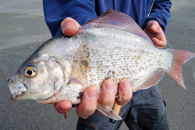
A redtail surfperch caught by a fisherman from a beach in San Diego, CA. These fish are thought to be common prey of coastal bottlenose dolphins. (Image Source: FishwithJD)

Diet studies on the offshore ecotype of bottlenose dolphins worldwide show a preference for cephalopods, similar to other toothed cetaceans who occupy similar regions, such as Risso’s dolphin, sperm whales, and pilot whales (Clarke 1986, Cockcroft and Ross 1990, Gonzalez et al. 1994, Barros et al. 2000, Walker et al. 1999). Because these animals seldom strand on accessible beaches, stomach contents analyses are limited to few studies and isotope analysis is more widely available from biopsies. We know these dolphins are sighted in deeper waters than the habitat of coastal dolphins where there are fewer nutrient plumes, so it is reasonable to hypothesize that the offshore ecotype consumes different species and may be more specialized than the coastal ecotype.
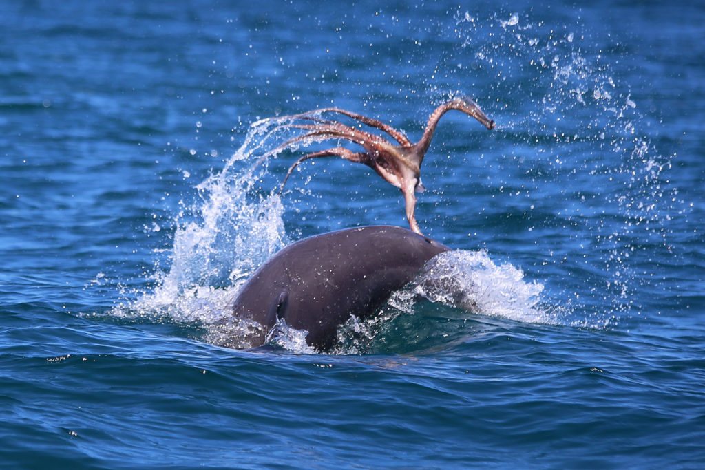
An bottlenose dolphin forages on an octopus. (Image source: Mandurah Cruises)

For a species that is so often observed from shore and boats, and is known for its charisma, it may be surprising that the diets of both the coastal and offshore bottlenose dolphins are still largely unknown. Such is the challenge of studying animals that live and feed underwater. I wish I could simply ask a dolphin, much like I would ask staff at restaurants: what is on the menu today? But, unfortunately, that is not possible. Instead, we must make educated hypotheses about the diets of both ecotypes based on necropsies and stable isotope studies, and behavioral and spatial surveys. And, I will continue to look to new technologies and creative thinking to provide the answers we are seeking.

Literature cited:

Ballance, L. T. (1992). Habitat use patterns and ranges of the bottlenose dolphin in the Gulf of California, Mexico. Marine Mammal Science8(3), 262-274.

Barros, N.B., and D. K. Odell. (1990). Food habits of bottlenose dolphins in the southeastern United States. Pages 309-328 in S. Leatherwood and R. R. Reeves, eds. The bottlenose dolphin. Academic Press, San Diego, CA.

Barros, N., E. Parsons and T. Jefferson. (2000). Prey of bottlenose dolphins from the South China Sea. Aquatic Mammals 26:2–6.

Clarke, M. 1986. Cephalopods in the diet of odontocetes. Pages 281–321 in M. Bryden and R. Harrison, eds. Research on dolphins. Clarendon Press, Oxford, NY.

Cockcroft, V., and G. Ross. (1990). Food and feeding of the Indian Ocean bottlenose dolphin off southern Natal, South Africa. Pages 295–308 in S. Leatherwood and R. R. Reeves, eds. The bottlenose dolphin. Academic Press, San Diego, CA.

Defran, R. H., Weller, D. W., Kelly, D. L., & Espinosa, M. A. (1999). Range characteristics of Pacific coast bottlenose dolphins (Tursiops truncatus) in the Southern California Bight. Marine Mammal Science15(2), 381-393.

Díaz‐Gamboa, R. E., Gendron, D., & Busquets‐Vass, G. (2018). Isotopic niche width differentiation between common bottlenose dolphin ecotypes and sperm whales in the Gulf of California. Marine Mammal Science34(2), 440-457.

Gonzalez, A., A. Lopez, A. Guerra and A. Barreiro. (1994). Diets of marine mammals stranded on the northwestern Spanish Atlantic coast with special reference to Cephalopoda. Fisheries Research 21:179–191.

Hanson, M. T., and Defran, R. H. (1993). The behavior and feeding ecology of the Pacific coast bottlenose dolphin, Tursiops truncatus. Aquatic Mammals19, 127-127.

Norris, K. S., and J. H. Prescott. (1961). Observations on Pacific cetaceans of Californian and Mexican waters. University of California Publications of Zoology 63:29, 1-402.

Shane, S. H. (1990). Comparison of bottlenose dolphin behavior in Texas and Florida, with a critique of methods for studying dolphin behavior. Pages 541-558 in S. Leatherwood and R. R. Reeves, eds. The bottlenose dolphin. Academic Press, San Diego, CA.

Shane, S., R. Wells and B. Wursig. (1986). Ecology, behavior and social organization of bottlenose dolphin: A review. Marine Mammal Science 2:34–63.

Walker, W.A. (1981). Geographical variation in morphology and biology of the bottlenose dolphins (Tursiops) in the eastern North Pacific. NMFS/SWFC Administrative Report. No, LJ-91-03C.

Walker, J., C. Potter and S. Macko. (1999). The diets of modern and historic bottlenose dolphin populations reflected through stable isotopes. Marine Mammal Science 15:335–350.

Marine Mammal Observing: Standardization is key

By: Alexa Kownacki, Ph.D. Student, OSU Department of Fisheries and Wildlife, Geospatial Ecology of Marine Megafauna Lab

For the past two years, I’ve had the opportunity to be the marine mammal observer aboard the NOAA ship Bell M. Shimada for 10 days in May. Both trips covered transects in the Northern California Current Ecosystem during the same time of year, but things looked very different from my chair on the fly bridge. This trip, in particular, highlighted the importance of standardization, seeing as it was the second replicate of the same area. Other scientists and crew members repeatedly asked me the same questions that made me realize just how important it is to have standards in scientific practices and communicating them.

Northern right whale dolphin porpoising out of the water beside the ship while in transit. May 2019. Image source: Alexa Kownacki

The questions:

  1. What do you actually do here and why are you doing it?
  2. Is this year the same as last year in terms of weather, sightings, and transect locations?
  3. Did you expect to see greater or fewer sightings (number and diversity)?
  4. What is this Beaufort Sea State scale that you keep referring to?

All of these are important scientific questions that influence our hypothesis-testing research, survey methods, expected results, and potential conclusions. Although the entire science party aboard the ship conducted marine science, we all had our own specialties and sometimes only knew the basics, if that, about what the other person was doing. It became a perfect opportunity to share our science and standards across similar, but different fields.

Now, to answer those questions:

  1. a) What do you actually do here and b) why are you doing it?

a) As the only marine mammal observer, I stand watch during favorable weather conditions while the ship is in transit, scanning from 0 to 90 degrees off the starboard side (from the front of the ship to a right angle towards the right side when facing forwards). Meanwhile, an application on an iPad called SeaScribe, records the ship’s exact location every 15 seconds, even when no animal is sighted. This process allows for the collection of absence data, that is, data when no animals are present. The SeaScribe program records the survey lines, along with manual inputs that I add, including weather and observer information. When I spot a marine mammal, I immediately mark an exact location on a hand held GPS, use my binoculars to identify the species, and add information to the sighting on the SeaScribe program, such as species, distance to the sighted animal(s), the degree (angle) to the sighting, number of animals in a group, behavior, and direction if traveling.

b) Marine mammal observing serves many different purposes. In this case, observing collects information about what species are where at what time. By piggy-backing on these large-scale, offshore oceanographic NOAA surveys, we have the unique opportunity to survey along standardized transect lines during different times of the year. From replicate survey data, we can start to form an idea of which species use which areas and what oceanographic conditions may impact species distributions. Currently there is not much consistent marine mammal data collected over these offshore areas between Northern California and Washington State, so our work is aiming to fill this knowledge gap.

Alexa observing on the R/V Shimada in May 2019, all bundled up. Image Source: Alexa Kownacki

  1. What is this Beaufort Sea State scale that you keep referring to?

Great question! It took me a while to realize that this standard measuring tool to estimate wind speeds and sea conditions, is not commonly recognized even among other sea-goers. The Beaufort Sea State, or BSS, uses an empirical scale that ranges from 0-12 with 0 being no wind and calm seas, to 12 being hurricane-force winds with 45+ ft seas. It is frequently referenced by scientists in oceanography, marine science, and climate science as a universally-understood metric. The BSS was created in 1805 by Francis Beaufort, a hydrographer in the Royal Navy, to standardize weather conditions across the fleet of vessels. By the mid-1850s, the BSS was standardized to non-naval use for sailing vessels, and in 1916, expanded to include information specific to the seas and not the sails1. We in the marine mammal observation field constantly collect BSS information while on survey to measure the quality of survey conditions that may impact our observations. BSS data allows us to measure the extent of our survey range, both in the distance that we are likely to sight animals and also the likelihood of sighting anything. Therefore, the BSS scale gives us an important indication of how much absence data we have collected, in addition to presence data.

A description of the Beaufort Sea State Scale. Image source: National Weather Service.


  1. Is this year the same as last year in terms of weather, sightings, and transect locations?

The short answer is no. Observed differences in marine mammal sightings in terms of both species diversity and number of animals between years can be normal. There are many potential explanatory variables, from differences in currents, upwelling strength, El Nino index levels, water temperatures, or, what was obvious in this case: sighting conditions. The weather in May 2019 varied greatly from that in May 2018. Last year, I observed for nearly every day because the Beaufort Sea State (BSS) was frequently less than a four. However, this year, more often than not, the BSS greater than or equal to five. A BSS of 5 equates to approximately 17-21 knots of breeze with 6-foot waves and the water appears to have many “white horses” or pronounced white caps with sea spray. Additionally, mechanical issue with winches delayed and altered our transect locations. Therefore, although multiple transects from May 2018 were also surveyed during May 2019, there were a few lines that do not have data for both cruises.

May 2018 with a BSS 1

May 2019 with a BSS 6


  1. Did you expect to see greater or fewer sightings (number and diversity)?

Knowing that I had less favorable sighting conditions and less amount of effort observing this year, it is not surprising that I observed fewer marine mammals in total count and in species diversity. Even less surprising is that on the day with the best weather, where the BSS was less than a five, I recorded the most sightings with the highest species count. May 2018 felt a bit like a tropical vacation because we had surprisingly sunny days with mild winds, and during May 2019 we had some rough seas with gale force winds. Additionally, as an observer, I need to remove as much bias as possible. So, yes, I had hoped to see beaked whales or orca like I did in May 2018, but I was still pleasantly surprised when I spotted fin whales feeding in May 2019.

Marine Mammal Species Number of Sightings
May 2018 May 2019
Humpback whale 31 6
Northern right whale dolphin 1 2
Pacific white-sided dolphin 3 6
UNID beaked whale 1 0
Cuvier’s beaked whale 1 0
Gray whale 4 1
Minke whale 1 1
Fin whale 4 1
Blue whale 1 0
Transient killer whale 1 0
Dall’s porpoise 2 0
Northern fur seal 1 0
California sea lion 0 1

Pacific white-sided dolphin. Image source: Alexa Kownacki

Standardization is a common theme. Observing between years on standard transects, at set speeds, in different conditions using standardized tools is critical to collecting high quality data that is comparable across different periods. Scientists constantly think about quality control. We look for trends and patterns, similarities and differences, but none of those could be understood without having standard metrics.

The entire science party aboard the R/V Shimada in May 2019, including a marine mammal scientist, phytoplankton scientists, zooplankton scientists, and fisheries scientists, and oceanographers. Image Source: Alexa Kownacki

Literature Cited:

1Oliver, John E. (2005). Encyclopedia of world climatology. Springer.


Data Wrangling to Assess Data Availability: A Data Detective at Work

By Alexa Kownacki, Ph.D. Student, OSU Department of Fisheries and Wildlife, Geospatial Ecology of Marine Megafauna Lab

Data wrangling, in my own loose definition, is the necessary combination of both data selection and data collection. Wrangling your data requires accessing then assessing your data. Data collection is just what it sounds like: gathering all data points necessary for your project. Data selection is the process of cleaning and trimming data for final analyses; it is a whole new bag of worms that requires decision-making and critical thinking. During this process of data wrangling, I discovered there are two major avenues to obtain data: 1) you collect it, which frequently requires an exorbitant amount of time in the field, in the lab, and/or behind a computer, or 2) other people have already collected it, and through collaboration you put it to a good use (often a different use then its initial intent). The latter approach may result in the collection of so much data that you must decide which data should be included to answer your hypotheses. This process of data wrangling is the hurdle I am facing at this moment. I feel like I am a data detective.

Data wrangling illustrated by members of the R-programming community. (Image source: R-bloggers.com)

My project focuses on assessing the health conditions of the two ecotypes of bottlenose dolphins between the waters off of Ensenada, Baja California, Mexico to San Francisco, California, USA between 1981-2015. During the government shutdown, much of my data was inaccessible, seeing as it was in possession of my collaborators at federal agencies. However, now that the shutdown is over, my data is flowing in, and my questions are piling up. I can now begin to look at where these animals have been sighted over the past decades, which ecotypes have higher contaminant levels in their blubber, which animals have higher stress levels and if these are related to geospatial location, where animals are more susceptible to human disturbance, if sex plays a role in stress or contaminant load levels, which environmental variables influence stress levels and contaminant levels, and more!

Alexa, alongside collaborators, photographing transiting bottlenose dolphins along the coastline near Santa Barbara, CA in 2015 as part of the data collection process. (Image source: Nick Kellar).

Over the last two weeks, I was emailed three separate Excel spreadsheets representing three datasets, that contain partially overlapping data. If Microsoft Access is foreign to you, I would compare this dilemma to a very confusing exam question of “matching the word with the definition”, except with the words being in different languages from the definitions. If you have used Microsoft Access databases, you probably know the system of querying and matching data in different databases. Well, imagine trying to do this with Excel spreadsheets because the databases are not linked. Now you can see why I need to take a data management course and start using platforms other than Excel to manage my data.

A visual interpretation of trying to combine datasets being like matching the English definition to the Spanish translation. (Image source: Enchanted Learning)

In the first dataset, there are 6,136 sightings of Common bottlenose dolphins (Tursiops truncatus) documented in my study area. Some years have no sightings, some years have fewer than 100 sightings, and other years have over 500 sightings. In another dataset, there are 398 bottlenose dolphin biopsy samples collected between the years of 1992-2016 in a genetics database that can provide the sex of the animal. The final dataset contains records of 774 bottlenose dolphin biopsy samples collected between 1993-2018 that could be tested for hormone and/or contaminant levels. Some of these samples have identification numbers that can be matched to the other dataset. Within these cross-reference matches there are conflicting data in terms of amount of tissue remaining for analyses. Sorting these conflicts out will involve more digging from my end and additional communication with collaborators: data wrangling at its best. Circling back to what I mentioned in the beginning of this post, this data was collected by other people over decades and the collection methods were not standardized for my project. I benefit from years of data collection by other scientists and I am grateful for all of their hard work. However, now my hard work begins.

The cutest part of data wrangling: finding adorable images of bottlenose dolphins, photographed during a coastal survey. (Image source: Alexa Kownacki).

There is also a large amount of data that I downloaded from federally-maintained websites. For example, dolphin sighting data from research cruises are available for public access from the OBIS (Ocean Biogeographic Information System) Sea Map website. It boasts 5,927,551 records from 1,096 data sets containing information on 711 species with the help of 410 collaborators. This website is incredible as it allows you to search through different data criteria and then download the data in a variety of formats and contains an interactive map of the data. You can explore this at your leisure, but I want to point out the sheer amount of data. In my case, the OBIS Sea Map website is only one major platform that contains many sources of data that has already been collected, not specifically for me or my project, but will be utilized. As a follow-up to using data collected by other scientists, it is critical to give credit where credit is due. One of the benefits of using this website, is there is information about how to properly credit the collaborators when downloading data. See below for an example:

Example citation for a dataset (Dataset ID: 1201):

Lockhart, G.G., DiGiovanni Jr., R.A., DePerte, A.M. 2014. Virginia and Maryland Sea Turtle Research and Conservation Initiative Aerial Survey Sightings, May 2011 through July 2013. Downloaded from OBIS-SEAMAP (http://seamap.env.duke.edu/dataset/1201) on xxxx-xx-xx.

Citation for OBIS-SEAMAP:

Halpin, P.N., A.J. Read, E. Fujioka, B.D. Best, B. Donnelly, L.J. Hazen, C. Kot, K. Urian, E. LaBrecque, A. Dimatteo, J. Cleary, C. Good, L.B. Crowder, and K.D. Hyrenbach. 2009. OBIS-SEAMAP: The world data center for marine mammal, sea bird, and sea turtle distributions. Oceanography 22(2):104-115

Another federally-maintained data source that boasts more data than I can quantify is the well-known ERDDAP website. After a few Google searches, I finally discovered that the acronym stands for Environmental Research Division’s Data Access Program. Essentially, this the holy grail of environmental data for marine scientists. I have downloaded so much data from this website that Excel cannot open the csv files. Here is yet another reason why young scientists, like myself, need to transition out of using Excel and into data management systems that are developed to handle large-scale datasets. Everything from daily sea surface temperatures collected on every, one-degree of latitude and longitude line from 1981-2015 over my entire study site to Ekman transport levels taken every six hours on every longitudinal degree line over my study area. I will add some environmental variables in species distribution models to see which account for the largest amount of variability in my data. The next step in data selection begins with statistics. It is important to find if there are highly correlated environmental factors prior to modeling data. Learn more about fitting cetacean data to models here.

The ERDAPP website combined all of the average Sea Surface Temperatures collected daily from 1981-2018 over my study site into a graphical display of monthly composites. (Image Source: ERDDAP)

As you can imagine, this amount of data from many sources and collaborators is equal parts daunting and exhilarating. Before I even begin the process of determining the spatial and temporal spread of dolphin sightings data, I have to identify which data points have sex identified from either hormone levels or genetics, which data points have contaminants levels already quantified, which samples still have tissue available for additional testing, and so on. Once I have cleaned up the datasets, I will import the data into the R programming package. Then I can visualize my data in plots, charts, and graphs; this will help me identify outliers and potential challenges with my data, and, hopefully, start to see answers to my focal questions. Only then, can I dive into the deep and exciting waters of species distribution modeling and more advanced statistical analyses. This is data wrangling and I am the data detective.

What people may think a ‘data detective’ looks like, when, in reality, it is a person sitting at a computer. (Image source: Elder Research)

Like the well-known phrase, “With great power comes great responsibility”, I believe that with great data, comes great responsibility, because data is power. It is up to me as the scientist to decide which data is most powerful at answering my questions.

Data is information. Information is knowledge. Knowledge is power. (Image source: thedatachick.com)


Over the Ocean and Under the Bridges: STEM Cruise on the R/V Oceanus

By Alexa Kownacki, Ph.D. Student, OSU Department of Fisheries and Wildlife, Geospatial Ecology of Marine Megafauna Lab

From September 22nd through 30th, the GEMM Lab participated in a STEM research cruise aboard the R/V Oceanus, Oregon State University’s (OSU) largest research vessel, which served as a fully-functioning, floating, research laboratory and field station. The STEM cruise focused on integrating science, technology, engineering and mathematics (STEM) into hands-on teaching experiences alongside professionals in the marine sciences. The official science crew consisted of high school teachers and students, community college students, and Oregon State University graduate students and professors. As with a usual research cruise, there was ample set-up, data collection, data entry, experimentation, successes, and failures. And because everyone in the science party actively participated in the research process, everyone also experienced these successes, failures, and moments of inspiration.

The science party enjoying the sunset from the aft deck with the Astoria-Megler bridge in the background. (Image source: Alexa Kownacki)

Dr. Leigh Torres, Dr. Rachael Orben, and I were all primarily stationed on flybridge—one deck above the bridge—fully exposed to the elements, at the highest possible location on the ship for best viewing. We scanned the seas in hopes of spotting a blow, a splash, or any sign of a marine mammal or seabird. Beside us, students and teachers donned binoculars and positioned themselves around the mast, with Leigh and I taking a 90-degree swath from the mast—either to starboard or to port. For those who had not been part of marine mammal observations previously, it was a crash course into the peaks and troughs—of both the waves and of the sightings. We emphasized the importance of absence data: knowledge of what is not “there” is equally as important as what is. Fortunately, Leigh chose a course that proved to have surprisingly excellent environmental conditions and amazing sightings. Therefore, we collected a large amount of presence data: data collected when marine mammals or seabirds are present.

High school student, Chris Quashnick Holloway, records a seabird sighting for observer, Dr. Rachael Orben. (Image source: Alexa Kownacki).

When someone sighted a whale that surfaced regularly, we assessed the conditions: the sea state, the animal’s behavior, the wind conditions, etc. If we deemed them as “good to fly”, our licensed drone pilot and Orange Coast Community College student, Jason, prepared his Phantom 4 drone. While he and Leigh set up drone operations, I and the other science team members maintained a visual on the whale and stayed in constant communication with the bridge via radio. When the drone was ready, and the bridge gave the “all clear”, Jason launched his drone from the aft deck. Then, someone tossed an unassuming, meter-long, wood plank overboard—keeping it attached to the ship with a line. This wood board serves as a calibration tool; the drone flies over it at varying heights as determined by its built-in altimeter. Later, we analyze how many pixels one meter occupied at different heights and can thereby determine the body length of the whale from still images by converting pixel length to a metric unit.

High school student, Alishia Keller, uses binoculars to observe a whale, while PhD student, Alexa Kownacki, radios updates on the whale’s location to the bridge and the aft deck. (Image source: Tracy Crews)

Finally, when the drone is calibrated, I radio the most recent location of our animal. For example, “Blow at 9 o’clock, 250 meters away”. Then, the bridge and I constantly adjust the ship’s speed and location. If the whale “flukes” (dives and exposes the ventral side of its tail), and later resurfaced 500 meters away at our 10 o’clock, I might radio to the bridge to, “turn 60 degrees to port and increase speed to 5 knots”. (See the Hidden Math Lesson below). Jason then positions the drone over the whale, adjusting the camera angle as necessary, and recording high-quality video footage for later analysis. The aerial viewpoint provides major advantages. Whales usually expose about 10 percent of their body above the water’s surface. However, with an aerial vantage point, we can see more of the whale and its surroundings. From here, we can observe behaviors that are otherwise obscured (Torres et al. 2018), and record footage that to help quantify body condition (i.e. lengths and girths). Prior to the batteries running low, Jason returns the drone back to the aft deck, the vessel comes to an idle, and Leigh catches the drone. Throughout these operations, those of us on the flybridge photograph flukes for identification and document any behaviors we observe. Later, we match the whale we sighted to the whale that the drone flew over, and then to prior sightings of this same individual—adding information like body condition or the presence of a calf. I like to think of it as whale detective work. Moreover, it is a team effort; everyone has a critical role in the mission. When it’s all said and done, this noninvasive approach provides life history context to the health and behaviors of the animal.

Drone pilot, Jason Miranda, flying his drone using his handheld ground station on the aft deck. (Photo source: Tracy Crews)

Hidden Math Lesson: The location of 10 o’clock and 60 degrees to port refer to the exact same direction. The bow of the ship is our 12 o’clock with the stern at our 6 o’clock; you always orient yourself in this manner when giving directions. The same goes for a compass measurement in degrees when relating the direction to the boat: the bow is 360/0. An angle measure between two consecutive numbers on a clock is: 360 degrees divided by 12-“hour” markers = 30 degrees. Therefore, 10 o’clock was 0 degrees – (2 “hours”)= 0 degrees- (2*30 degrees)= -60 degrees. A negative degree less than 180 refers to the port side (left).

Killer whale traveling northbound.

Our trip was chalked full of science and graced with cooperative weather conditions. There were more highlights than I could list in a single sitting. We towed zooplankton nets under the night sky while eating ice cream bars; we sang together at sunset and watched the atmospheric phenomena: the green flash; we witnessed a humpback lunge-feeding beside the ship’s bow; and we saw a sperm whale traveling across calm seas.

Sperm whale surfacing before a long dive.

On this cruise, our lab focused on the marine mammal observations—which proved excellent during the cruise. In only four days of surveying, we had 43 marine mammal sightings containing 362 individuals representing 9 species (See figure 1). As you can see from figure 2, we traveled over shallow, coastal and deep waters, in both Washington and Oregon before inland to Portland, OR. Because we ventured to areas with different bathymetric and oceanographic conditions, we increased our likelihood of seeing a higher diversity of species than we would if we stayed in a single depth or area.

Humpback whale lunge feeding off the bow.

Number of sightings Total number of individuals
Humpback whale 22 40
Pacific white-sided dolphin 3 249
Northern right whale dolphin 1 9
Killer whale 1 3
Dall’s porpoise 5 49
Sperm whale 1 1
Gray whale 1 1
Harbor seal 1 1
California sea lion 8 9
Total 43 362

Figure 1. Summary table of all species sightings during cruise while the science team observed from the flybridge.

Pacific white-sided dolphins swimming towards the vessel.

Figure 2. Map with inset displaying study area and sightings observed by species during the cruise, made in ArcMap. (Image source: Alexa Kownacki).

Even after two days of STEM outreach events in Portland, we were excited to incorporate more science. For the transit from Portland, OR to Newport, OR, the entire science team consisted two people: me and Jason. But even with poor weather conditions, we still used science to answer questions and help us along our journey—only with different goals than on our main leg. With the help of the marine technician, we set up a camera on the bow of the ship, facing aft to watch the vessel maneuver through the famous Portland bridges.

Video 1. Time-lapse footage of the R/V Oceanus maneuvering the Portland Bridges from a GoPro. Compiled by Alexa Kownacki, assisted by Jason Miranda and Kristin Beem.

Prior to the crossing the Columbia River bar and re-entering the Pacific Ocean, the R/V Oceanus maneuvered up the picturesque Columbia River. We used our geospatial skills to locate our fellow science team member and high school student, Chris, who was located on land. We tracked each other using GPS technology in our cell phones, until the ship got close enough to use natural landmarks as reference points, and finally we could use our binoculars to see Chris shining a light from shore. As the ship powered forward and passed under the famous Astoria-Megler bridge that connects Oregon to Washington, Chris drove over it; he directed us “100 degrees to port”. And, thanks to clear directions, bright visual aids, and spatiotemporal analysis, we managed to find our team member waving from shore. This is only one of many examples that show how in a few days at sea, students utilized new skills, such as marine mammal observational techniques, and honed them for additional applications.

On the bow, Alexa and Jason use binoculars to find Chris–over 4 miles–on the Washington side of the Columbia River. (Image source: Kristin Beem)

Great science is the result of teamwork, passion, and ingenuity. Working alongside students, teachers, and other, more-experienced scientists, provided everyone with opportunities to learn from each other. We created great science because we asked questions, we passed on our knowledge to the next person, and we did so with enthusiasm.

High school students, Jason and Chris, alongside Dr. Leigh Torres, all try to get a glimpse at the zooplankton under Dr. Kim Bernard’s microscope. (Image source: Tracy Crews).

Check out other blog posts written by the science team about the trip here.

The Recipe for a “Perfect” Marine Mammal and Seabird Cruise

By Alexa Kownacki, Ph.D. Student, OSU Department of Fisheries and Wildlife, Geospatial Ecology of Marine Megafauna Lab

Science—and fieldwork in particular—is known for its failures. There are websites, blogs, and Twitter pages dedicated to them. This is why, when things go according to plan, I rejoice. When they go even better than expected, I practically tear up from amazement. There is no perfect recipe for a great marine mammal and seabird research cruise, but I would suggest that one would look like this:

 A Great Marine Mammal and Seabird Research Cruise Recipe:

  • A heavy pour of fantastic weather
    • Light on the wind and seas
    • Light on the glare
  • Equal parts amazing crew and good communication
  • A splash of positivity
  • A dash of luck
  • A pinch of delicious food
  • Heaps of marine mammal and seabird sightings
  • Heat to approximately 55-80 degrees F and transit for 10 days along transects at 10-12 knots

The end of another beautiful day at sea on the R/V Shimada. Image source: Alexa K.

The Northern California Current Ecosystem (NCCE) is a highly productive area that is home to a wide variety of cetacean species. Many cetaceans are indicator species of ecosystem health as they consume large quantities of prey from different levels in trophic webs and inhabit diverse areas—from deep-diving beaked whales to gray whales traveling thousands of miles along the eastern north Pacific Ocean. Because cetacean surveys are a predominant survey method in large bodies of water, they can be extremely costly. One alternative to dedicated cetacean surveys is using other research vessels as research platforms and effort becomes transect-based and opportunistic—with less flexibility to deviate from predetermined transects. This decreases expenses, creates collaborative research opportunities, and reduces interference in animal behavior as they are never pursued. Observing animals from large, motorized, research vessels (>100ft) at a steady, significant speed (>10kts/hour), provides a baseline for future, joint research efforts. The NCCE is regularly surveyed by government agencies and institutions on transects that have been repeated nearly every season for decades. This historical data provides critical context for environmental and oceanographic dynamics that impact large ecosystems with commercial and recreational implications.

My research cruise took place aboard the 208.5-foot R/V Bell M. Shimada in the first two weeks of May. The cruise was designated for monitoring the NCCE with the additional position of a marine mammal observer. The established guidelines did not allow for deviation from the predetermined transects. Therefore, mammals were surveyed along preset transects. The ship left port in San Francisco, CA and traveled as far north as Cape Meares, OR. The transects ranged from one nautical mile from shore and two hundred miles offshore. Observations occurred during “on effort” which was defined as when the ship was in transit and moving at a speed above 8 knots per hour dependent upon sea state and visibility. All observations took place on the flybridge during conducive weather conditions and in the bridge (one deck below the flybridge) when excessive precipitation was present. The starboard forward quarter: zero to ninety degrees was surveyed—based on the ship’s direction (with the bow at zero degrees). Both naked eye and 7×50 binoculars were used with at least 30 percent of time binoculars in use. To decrease observer fatigue, which could result in fewer detected sightings, the observer (me) rotated on a 40 minutes “on effort”, 20 minutes “off effort” cycle during long transits (>90 minutes).

Alexa on-effort using binoculars to estimate the distance and bearing of a marine mammal sighted off the starboard bow. Image source: Alexa K.

Data was collected using modifications to the SEEbird Wincruz computer program on a ruggedized laptop and a GPS unit was attached. At the beginning of each day and upon changes in conditions, the ship’s heading, weather conditions, visibility, cloud cover, swell height, swell direction, and Beaufort sea state (BSS) were recorded. Once the BSS or visibility was worse than a “5” (1 is “perfect” and 5 is “very poor”) observations ceased until there was improvement in weather. When a marine mammal was sighted the latitude and longitude were recorded with the exact time stamp. Then, I noted how the animal was sighted—either with binoculars or naked eye—and what action was originally noticed—blow, splash, bird, etc. The bearing and distance were noted using binoculars. The animal was given three generalized behavior categories: traveling, feeding, or milling. A sighting was defined as any marine mammal or group of animals. Therefore, a single sighting would have the species and the best, high, and low estimates for group size.

By my definitions, I had the research cruise of my dreams. There were moments when I imagined people joining this trip as a vacation. I *almost* felt guilty. Then, I remember that after watching water for almost 14 hours (thanks to the amazing weather conditions), I worked on data and reports and class work until midnight. That’s the part that no one talks about: the data. Fieldwork is about collecting data. It’s both what I live for and what makes me nervous. The amount of time, effort, and money that is poured into fieldwork is enormous. The acquisition of the data is not as simple as it seems. When I briefly described my position on this research cruise to friends, they interpret it to be something akin to whale-watching. To some extent, this is true. But largely, it’s grueling hours that leave you fatigued. The differences between fieldwork and what I’ll refer to as “everything else” AKA data analysis, proposal writing, manuscript writing, literature reviewing, lab work, and classwork, are the unbroken smile, the vaguely tanned skin, the hours of laughter, the sea spray, and the magical moments that reassure me that I’ve chosen the correct career path.

Alexa photographing a gray whale at sunset near Newport, OR. Image source: Alexa K.

This cruise was the second leg of the Northern California Current Ecosystem (NCCE) survey, I was the sole Marine Mammal and Seabird Observer—a coveted position. Every morning, I would wake up at 0530hrs, grab some breakfast, and climb to the highest deck: the fly-bridge. Akin to being on the top of the world, the fly-bridge has the best views for the widest span. From 0600hrs to 2000hrs I sat, stood, or danced in a one-meter by one-meter corner of the fly-bridge and surveyed. This visual is why people think I’m whale watching. In reality, I am constantly busy. Nonetheless, I had weather and seas that scientists dream about—and for 10 days! To contrast my luck, you can read Florence’s blog about her cruise. On these same transects, in February, Florence experienced 20-foot seas with heavy rain with very few marine mammal sightings—and of those, the only cetaceans she observed were gray whales close to shore. That starkly contrasts my 10 cetacean species with upwards of 45 sightings and my 20-minute hammock power naps on the fly-bridge under the warm sun.

Pacific white-sided dolphins traveling nearby. Image source: Alexa K.

Marine mammal sightings from this cruise included 10 cetacean species: Pacific white-sided dolphin, Dall’s porpoise, unidentified beaked whale, Cuvier’s beaked whale, gray whale, Minke whale, fin whale, Northern right whale dolphin, blue whale, humpback whale, and transient killer whale and one pinniped species: northern fur seal. What better way to illustrate these sightings than with a map? We are a geospatial lab after all.

Cetacean Sightings on the NCCE Cruise in May 2018. Image source: Alexa K.

This map is the result of data collection. However, it does not capture everything that was observed: sea state, weather, ocean conditions, bathymetry, nutrient levels, etc. There are many variables that can be added to maps–like this one (thanks to my GIS classes I can start adding layers!)–that can provide a better understanding of the ecosystem, predator-prey dynamics, animal behavior, and population health.

The catch from a bottom trawl at a station with some fish and a lot of pyrosomes (pink tube-like creatures). Image source: Alexa K.

Being a Ph.D. student can be physically and mentally demanding. So, when I was offered the opportunity to hone my data collection skills, I leapt for it. I’m happiest in the field: the wind in my face, the sunshine on my back, surrounded by cetaceans, and filled with the knowledge that I’m following my passion—and that this data is contributing to the greater scientific community.

Humpback whale photographed traveling southbound. Image source: Alexa K.

Managing Oceans: the inner-workings of marine policy

By Alexa Kownacki, Ph.D. Student, OSU Department of Fisheries and Wildlife, Geospatial Ecology of Marine Megafauna Lab

When we hear “marine policy” we broadly lump it together with environmental policy. However, marine ecosystems differ greatly from their terrestrial counterparts. We wouldn’t manage a forest like an ocean, nor would we manage an ocean like a forest. Why not? The answer to this question is complex and involves everything from ecology to politics.

Oceans do not have borders; they are fluid and dynamic. Interestingly, by defining marine ecosystems we are applying some kind of borders. But water (and all its natural and unnatural content) flows between these ‘ecosystems’. Marine ecosystems are home to a variety of anthropogenic activities such as transportation and recreation, in addition to an abundance of species that represent the three major domains of biology: Archaea, Bacteria, and Eukarya. Humans are the only creatures who “recognize” the borders that policymakers and policy actors have instilled. A migrating gray whale does not have a passport stamped as it travels from its breeding grounds in Mexican waters to its feeding grounds in the Gulf of Alaska. In contrast, a large cargo ship—or even a small sailing vessel—that crosses those boundaries is subjected to a series of immigration checkpoints. Combining these human and the non-human facets makes marine policy complex and variable.

The eastern Pacific gray whale migration route includes waters off of Mexico, Canada, and the United States. Source: https://www.learner.org/jnorth/tm/gwhale/annual/map.html

Environmental policy of any kind can be challenging. Marine environmental policy adds many more convoluted layers in terms of unknowns; marine ecosystems are understudied relative to terrestrial ecosystems and therefore have less research conducted on how to best manage them. Additionally, there are more hands in the cookie jar, so to speak; more governments and more stakeholders with more opinions (Leslie and McLeod 2007). So, with fewer examples of successful ecosystem-based management in coastal and marine environments and more institutions with varied goals, marine ecosystems become challenging to manage and monitor.

A visual representation of what can happen when there are many groups with different goals: no one can easily get what they want. Image Source: The Brew Monks

With this in mind, it is understandable that there is no official manual on policy development.  There is, however, a broadly standardized process of how to develop, implement, and evaluate environmental policies: 1) recognize a problem 2) propose a solution 3) choose a solution 4) put the solution into effect and 4) monitor the results (Zacharias pp. 16-21). For a policy to be deemed successful, specific criteria must be met, which means that a common policy is necessary for implementation and enforcement. Within the United States, there are a multiple governing bodies that protect the ocean, including the National Oceanic and Atmospheric Administration (NOAA), Environmental Protection Agency (EPA), Fish and Wildlife Service (USFWS), and the Department of Defense (DoD)—all of which have different mission statements, budgets, and proposals. To create effective environmental policies, collaboration between various groups is imperative. Nevertheless, bringing these groups together, even those within the same nation, requires time, money, and flexibility.

This is not to say that environmental policy for terrestrial systems, but there are fewer moving parts to manage. For example, a forest in the United States would likely not be an international jurisdiction case because the borders are permanent lines and national management does not overlap. However, at a state level, jurisdiction may overlap with potentially conflicting agendas. A critical difference in management strategies is preservation versus conservation. Preservation focuses on protecting nature from use and discourages altering the environment. Conservation, centers on wise-use practices that allow for proper human use of environments such as resource use for economic groups. One environmental group may believe in preservation, while one government agency may believe in conservation, creating friction amongst how the land should be used: timber harvest, public use, private purchasing, etc.

Linear representation of preservation versus conservation versus exploitation. Image Source: Raoof Mostafazadeh

Furthermore, a terrestrial forest has distinct edges with measurable and observable qualities; it possesses intrinsic and extrinsic values that are broadly recognized because humans have been utilizing them for centuries. Intrinsic values are things that people can monetize, such as commercial fisheries or timber harvests whereas extrinsic values are things that are challenging to put an actual price on in terms of biological diversity, such as the enjoyment of nature or the role of species in pest management; extrinsic values generally have a high level of human subjectivity because the context of that “resource” in question varies upon circumstances (White 2013). Humans are more likely to align positively with conservation policies if there are extrinsic benefits to them; therefore, anthropocentric values associated with the resources are protected (Rode et al. 2015). Hence, when creating marine policy, monetary values are often placed on the resources, but marine environments are less well-studied due to lack of accessibility and funding, making any valuation very challenging.

The differences between direct (intrinsic) versus indirect (extrinsic) values to biodiversity that factor into environmental policy. Image Source: Conservationscienceblog.wordpress.com

Assigning a cost or benefit to environmental services is subjective (Dearborn and Kark 2010). What is the benefit to a child seeing an endangered killer whale for the first time? One could argue priceless. In order for conservation measures to be implemented, values—intrinsic and extrinsic—are assigned to the goods and services that the marine environment provides—such as seafood and how the ocean functions as a carbon sink. Based off of the four main criteria used to evaluate policy, the true issue becomes assessing the merit and worth. There is an often-overlooked flaw with policy models: it assumes rational behavior (Zacharias 126). Policy involves relationships and opinions, not only the scientific facts that inform them; this is true in terrestrial and marine environments. People have their own agendas that influence, not only the policies themselves, but the speed at which they are proposed and implemented.

Tourists aboard a whale-watching vessel off of the San Juan Islands, enjoying orca in the wild. Image Source: Seattle Orca Whale Watching

One example of how marine policy evolves is through groups, such as the International Whaling Commission, that gather to discuss such policies while representing many different stakeholders. Some cultures value the whale for food, others for its contributions to the surrounding ecosystems—such as supporting healthy seafood populations. Valuing one over the other goes beyond a monetary value and delves deeper into the cultures, politics, economics, and ethics. Subjectivity is the name of the game in environmental policy, and, in marine environmental policy, there are many factors unaccounted for, that decision-making is incredibly challenging.

Efficacy in terms of the public policy for marine systems presents a challenge because policy happens slowly, as does research. There is no equation that fits all problems because the variables are different and dynamic; they change based on the situation and can be unpredictable. When comparing institutional versus impact effectiveness, they both are hard to measure without concrete goals (Leslie and McLeod 2007). Marine ecosystems are open environments which add an additional hurdle: setting measurable and achievable goals. Terrestrial environments contain resources that more people utilize, more frequently, and therefore have more set goals. Without a problem and potential solution there is no policy. Terrestrial systems have problems that humans recognize. Marine systems have problems that are not as visible to people on a daily basis. Therefore, terrestrial systems have more solutions presented to mitigate problems and more policies enacted.

As marine scientists, we don’t always immediately consider how marine policy impacts our research. In the case of my project, marine policy is something I constantly have to consider. Common bottlenose dolphins are protected under the Marine Mammal Protection Act (MMPA) and inhabit coastal of both the United States and Mexico, including within some Marine Protected Areas (MPA). In addition, some funding for the project comes from NOAA and the DoD. Even on the surface-level it is clear that policy is something we must consider as marine scientists—whether we want to or not. We may do our best to inform policymakers with results and education based on our research, but marine policy requires value-based judgements based on politics, economics, and human objectivity—all of which are challenging to harmonize into a succinct problem with a clear solution.

Two common bottlenose dolphins (coastal ecotype) traveling along the Santa Barbara, CA shoreline. Image Source: Alexa Kownacki

References:

Dearborn, D. C. and Kark, S. 2010. Motivations for Conserving Urban Biodiversity. Conservation Biology, 24: 432-440. doi:10.1111/j.1523-1739.2009.01328.x

Leslie, H. M. and McLeod, K. L. (2007), Confronting the challenges of implementing marine ecosystem‐based management. Frontiers in Ecology and the Environment, 5: 540-548. doi:10.1890/060093

Munguia, P., and A. F. Ojanguren. 2015. Bridging the gap in marine and terrestrial studies. Ecosphere 6(2):25. http://dx.doi.org/10.1890/ES14-00231.1

Rode, J., Gomez-Baggethun, E., Krause, M., 2015. Motivation crowding by economic payments in conservation policy: a review of the empirical evidence. Ecol. Econ. 117, 270–282 (in this issue).

White, P. S. (2013), Derivation of the Extrinsic Values of Biological Diversity from Its Intrinsic Value and of Both from the First Principles of Evolution. Conservation Biology, 27: 1279-1285. doi:10.1111/cobi.12125

Zacharias, M. 2014. Marine Policy. London: Routledge.


A porpoise-full lesson on cetacean identification

By Amanda Holdman, M.S. student

The rain is beginning to lighten, the heavy winds are starting  to dissipate, and the sun is beginning to shine. Seabirds are starting to fill the air and marine mammals are starting to fill the coastline, making this week a perfect time to learn about some of the small, cryptic cetaceans that consider the Oregon coast home year round.

While I was walking my dog on South Beach in Newport last week, I heard the mother of a small family point and shout that she had just seen an animal that she referred to as a “porpoise/dolphin/small whale.” Upon a second sighting of it, she ruled against the small whale and decided on a dolphin. In reality, she had just sighted a harbor porpoise.

Throughout the duration of my work with Oregon State studying the patterns of harbor porpoise occurrence, one of the most frequently asked questions I get is “What is the difference between a porpoise and a dolphin?”

Differentiating between a dolphin and porpoise is probably the most common identification mistake when it comes to cetaceans. Understandably, there is significant confusion between the two species. The words dolphin and porpoise were, colloquially, used as synonyms until the 1970’s. Unlike lions and tigers that are not only in the same family, but also the same genus, dolphins and porpoises are in different families, having diverged evolutionarily about 15 million years ago! Therefore, dolphins and porpoises are more distinct than lions and tigers. These differences span from head and fin shape, to behavior, group size and vocals.

Physical Differences

Most people are quite certain they are seeing a dolphin mainly because dolphins are more prevalent than porpoises; over 30 species of dolphins are known to exist, but only 6 porpoise species have been identified worldwide. Unless, you’ve seen dolphins and porpoises side by side, nose to fin, it is quite difficult to tell the difference at first glance. In the natural history of cetacean’s course at Oregon State, we are taught that the three main visual differences are in the shape of the teeth, snout, and dorsal fin. But in reality, the first two characteristics aren’t likely to help you spot them from shore. In addition to fin size, the behavior and group size is more likely to cue you in on what animal you are seeing. The picture below does a pretty good job summarizing their physical characteristics. Porpoise have a small triangle fin, while dolphins have more of a curved, pointy fin.

identificationDrawing by Mike Rock, 2009.

Size Differences

The lengths and widths of dolphins vary anywhere from 4 feet to 30 feet. Killer whales, the largest dolphin species and known predator to the harbor porpoise, can weigh up to ten tons, while the harbor porpoise is about five feet and rarely weighs in over 150 pounds.  Porpoises are one of the smallest cetaceans, and because of their small size, they lose body heat to the water more quickly than other cetaceans. Their blunt snout is likely an adaptation to minimize surface area to conserve heat. The small sizes of porpoise require them to eat frequently, rather than depending on fat reserves, making them more of an opportunistic feeder. The need to constantly forage also keeps harbor porpoise from migrating on a large scale. Harbor porpoise are known to move from onshore to offshore waters with changing water temperatures and prey distributions, but not known to make long migration trips.

Social Differences

Porpoises are also less social and talkative than dolphins. Dolphins are typically found in large groups, can be highly acrobatic, and often seen bow-riding. Porpoise, specifically harbor porpoise, are often found singularly or in groups of two to three, and shy away from vessels, making them difficult to observe at sea. While both species have large melon heads for echolocation purposes, dolphins make whistles through there blow holes to communicate with each other underwater. Evolutionary scientists believe porpoises do not whistle due to structural differences in their blowhole. (This is why acoustics is such a great way to learn about the occurrence patterns of harbor porpoise – their echolocation is very distinct!) Porpoise echolocation signals have evolved into a very narrow frequency range – theoretically to protect themselves from killer whale predation by echolocating at a frequency killer whales cannot hear.  Dolphins have evolved other strategies to avoid predators such as large group size and fast speed.

While differentiating between porpoises and dolphins takes a bit of practice, it is important to differentiate between the two species because we manage them differently due to some of their morphological differences. Their different adaptations between the species make them more sensitive to certain stressors. For example, for harbor porpoise, the sound produced from boat noise or renewable energy devices is more likely to impact them than other cetaceans. The sensitivity of the nerve cells in the ears of animals (including humans) generally corresponds to the frequencies that each animal produces. So animals like the harbor porpoise have more nerves in their ears that are tuned to very high frequencies (since they make high frequency sounds). If the nerve cells in the harbor porpoise ears become damaged, their ability to communicate, navigate and find food is seriously affected. In addition to their small home ranges and moderately high position in the food web, the sensitivity of harbor porpoise to ocean noise levels make harbor porpoise an important indicator species for ecosystem health, and an important species to study on the Oregon Coast.