How fat do baleen whales get? Recent publication shows how humpback whales increase their body condition over the foraging season. 

Dr. KC Bierlich, Postdoctoral Scholar, OSU Department of Fisheries, Wildlife, & Conservation Sciences, Geospatial Ecology of Marine Megafauna (GEMM) Lab

Traveling across oceans takes a lot of energy. Most baleen whales use stored energy acquired on their summer foraging grounds to support the costs of migration to and reproduction on their winter breeding grounds. Since little, if any, feeding takes place during the migration and winter season, it is essential that baleen whales obtain enough food to increase their fat reserves to support reproduction. As such, baleen whales are voracious feeders, and they typically depart the foraging grounds much fatter than when they had arrived. 

So, how fat do baleen whales typically get by the end of the foraging season, and how does this differ across reproductive classes, such as a juvenile female vs. a pregnant female? Understanding these questions is key for identifying what a typical “healthy” whale looks like, information which can then help scientists and managers monitor potential impacts from environmental and anthropogenic stressors. In this blog, I will discuss a recent publication in Frontiers in Marine Science (https://doi.org/10.3389/fmars.2022.1036860) that is from my PhD dissertation with the Duke University Marine Robotics and Remote Sensing (MaRRS) Lab, and also includes GEMM lab members Allison Dawn and Clara Bird. In this study, we analyzed how humpback whales (Megaptera novaeangliae) along the Western Antarctic Peninsula (WAP) increase their fat reserves throughout the austral summer foraging season (Bierlich et al., 2022). This work also helps provide insight to the GEMM Lab’s GRANITE project (Gray whale Response to Ambient Noise Informed by Technology and Ecology), where we are interested in how Pacific Coast Feeding Group (PCFG) gray whales increase their energy reserves in response to environmental variability and increasing human activities. 

Eastern South Pacific humpback whales, identified as Stock G by the International Whaling Commission, travel over 16,000 km between summer foraging grounds along the WAP and winter breeding grounds between Ecuador and Costa Rica (Fig. 1). Like most baleen whales, Stock G humpback whales were heavily exploited by 20th century commercial whaling. Recent evidence suggests that this population is recovering, with an estimated increase in population size of ~7,000 individuals in 2000 to ~19,107 in 2020 (Johannessen et al., 2022). 

However, there are long-term concerns for this population. The WAP is one of the fastest warming regions on the planet, and regional populations of krill, an important food source for humpback whales, have declined steeply over the past half-century. Additionally, the WAP has seen a rapid expansion of human activities, such as tourism and krill fishing. Specifically, the WAP has experienced an increase in tourism from a total of 6,700 visitors from 59 voyages in 1990 to 73,000 visitors from 408 voyages in 2020, which may be causing increased stress levels amongst Stock G (Pallin et al., 2022). Furthermore, the krill fishery has increased harvest activities in key foraging areas for humpback whales (Reisinger et al., 2022). Understanding how humpback whales increase their energy reserves over the course of the foraging season can help researchers establish a baseline to monitor future impacts from climate change and human activities. This work also provides an opportunity for comparisons to other baleen whale populations that are also exposed to multiple stressors, such as the PCFG gray whales off the Newport Coast who are constantly exposed to vessel traffic and at risk of entanglement from fishing gear. 

Figure 1. The migration route of the Stock G humpback whale population. Figure adapted from Whales of the Antarctic Peninsula Report, WWF 2018.

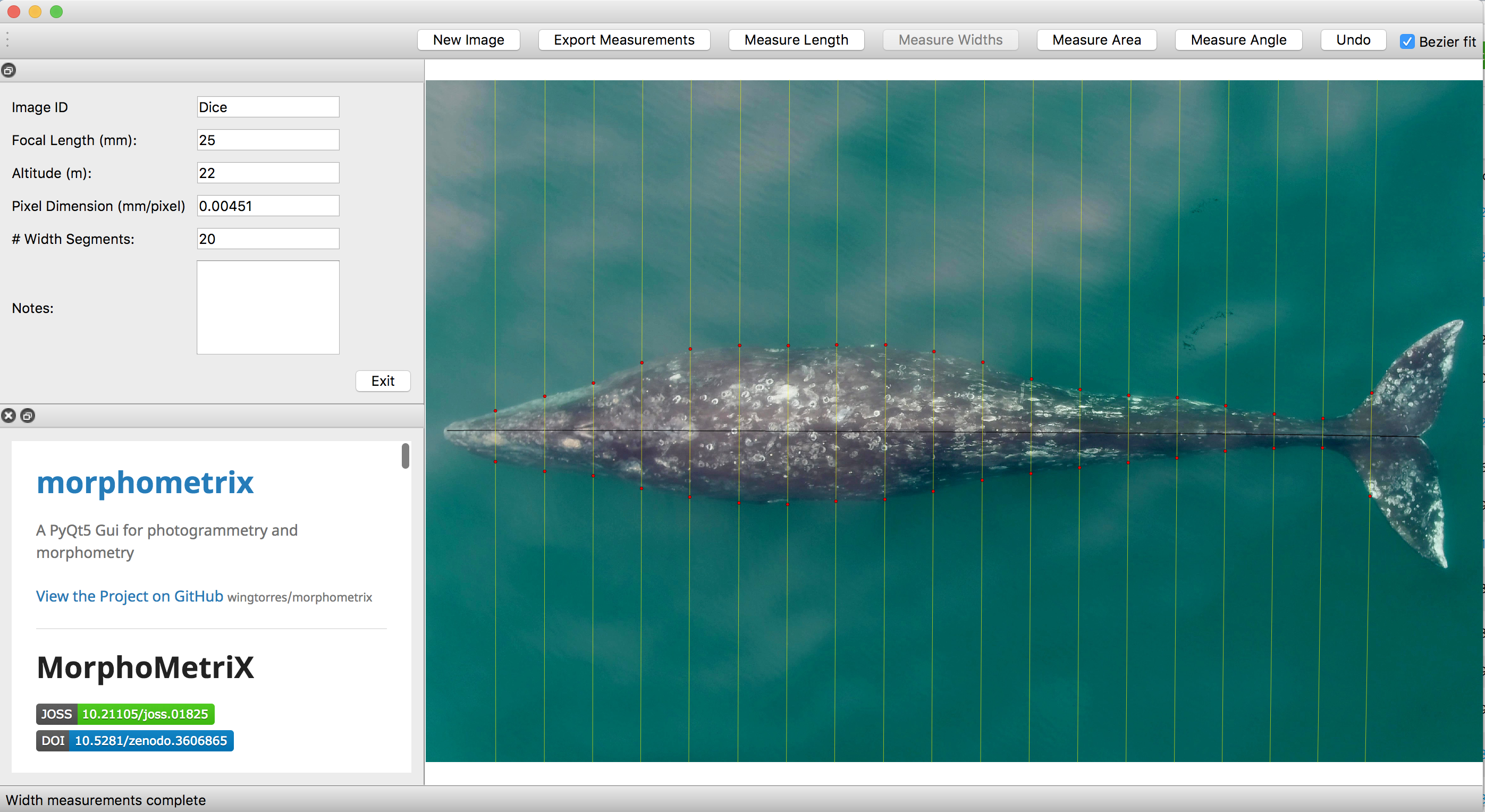
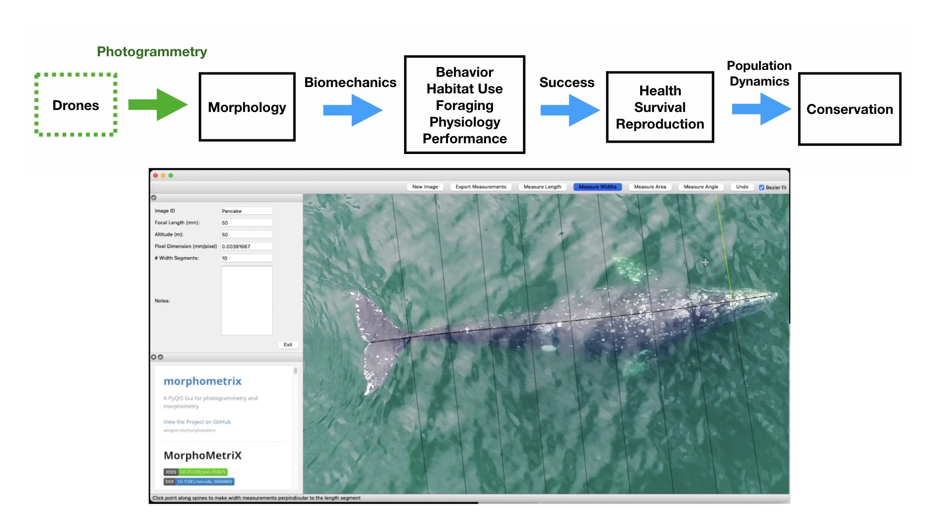
To understand how humpback whales increase their energy reserves throughout the foraging season, we collected drone imagery of whales along the WAP between November and June, 2017-2019 (Fig. 2). We used these images to measure the length and width of the whale to estimate body condition, which represents an animal’s relative energy reserve and can reflect foraging success (see previous blog). We collected drone imagery from a combination of research stations (Palmer Station), research vessels (Laurence M. Gould), and tour ships (One Ocean Expeditions). We used several different drones types and accounted for measurement uncertainty associated with the camera, focal length lens, altitude, and altimeter (barometer/LiDAR) from each drone (see previous blog and Bierlich et al., 2021a, 2021b). We also took biopsy samples to identify the sex of each individual and to determine if females were pregnant or not. 

Figure 2. Two humpbacks gracefully swimming in the chilly water along the Western Antarctic Peninsula. Photo taken by KC Bierlich & the Duke University Marine Robotics and Remote Sensing (MaRRS) Lab.

Our final dataset included body condition measurements for 228 total individuals. We found that body condition increased linearly between November and June for each reproductive class, which included calves, juvenile females, juvenile whales of unknown sex, lactating females, mature whales of unknown sex, and non-pregnant females (Fig. 3). This was an interesting finding because a recent publication analyzing tagged whales from the same population found that humpback whales have high foraging rates in early season that then significantly decrease by February and March (Nichols et al., 2022). So, despite these reduced foraging rates throughout the season, humpback whales continue to gain substantial mass into the late season. This continued increase in body condition implies a change in krill abundance and/or quality into the late season, which may compensate for the lower feeding rates. For example, krill density and biomass increases by over an order of magnitude across the season (Reiss et al., 2017) and their lipid content increases by ~4x (Hagen et al., 1996). Thus, humpback whales likely compensate for their lower feeding rates by feeding on denser and higher quality krill, ultimately increasing their efficiency in energy deposition. 

Figure 3. Body condition, here measured as Body Area Index (BAI), increases linearly for each reproductive class across the austral summer foraging season (Nov – June) for humpback whales along the Western Antarctic Peninsula. The shading represents the uncertainty around the estimated relationship. The colors represent the month of data collection.

We found that body condition increase varied amongst reproductive classes. For example, lactating females had the poorest measures of body condition across the season, reflecting the high energetic demands of nursing their calves (Fig. 3). Conversely, non-pregnant females had the highest body condition at the start of the season compared to all the other classes, likely reflecting the energy saved and recovered by skipping breeding that year.  Calves, juvenile whales, and mature whales all reached similar levels of body condition by the end of the season, though mature whales will likely invest most of their energy stores toward reproduction, whereas calves and juveniles likely invest toward growth. We also found a positive relationship between the total length of lactating females and their calves, suggesting that bigger moms have bigger calves (Fig. 4). A similar trend has also been observed in other baleen whale species including southern and North Atlantic right whales (Christiansen et al., 2018; Stewart et al., 2022).

Figure 4. Big mothers have big calves. Total length (TL) measurement between mother-calf pairs. The bars around each point represents the uncertainty (95% highest posterior density intervals). The colors represent the month of data collection. The blue line represents the best fit from a Deming regression, which incorporate measurement uncertainty in both the independent (mother’s TL) and dependent variable (calf’s TL).

The results from the humpback study provide insight for my current work exploring how PCFG gray whales increase their energy reserves in relation to environmental variability and increasing human activities. Over the past seven years, the GEMM Lab has been collecting drone images of PCFG gray whales off the coast of Oregon to measure their body condition (see this GRANITE Project blog). Many of the individuals we encounter are seen across years and throughout the foraging season, providing an opportunity to evaluate how an individual’s body condition is influenced by environmental variation, stress levels, maturity, and reproduction. For example, we had nine total body condition measurements of a female PCFG whale named “Sole”, who had a curvilinear increase in body condition throughout the summer foraging season – a rapid increase in early season that slowed as the season progressed (Fig. 5). This raises many questions for us: is this how most PCFG whales typically increase their body condition during the summer? Is this increase different for pregnant or lactating females? How is this increase impacted by environmental variability or anthropogenic stressors? Repeated measurements of individuals, in addition to Sole, in different reproductive classes across different years will help us determine what body condition is considered a healthy range for gray whales. This is particularly important for monitoring any potential health consequences from anthropogenic stressors, such as vessel noise and traffic (see recent blog by GEMM Lab alum Leila Lemos). We are currently analyzing body condition measurements between 2016 – 2022, so stay tuned for upcoming results!

Figure 6. Body condition, here measured as Body Area Index (BAI), increases curvilinearly for “Sole”, a mature female Pacific Coat Feeding Group gray whale, imaged nine times along the Oregon coast in 2021. The colors represent the month of data collection. 

References

Bierlich, K. C., Hewitt, J., Bird, C. N., Schick, R. S., Friedlaender, A., Torres, L. G., et al. (2021a). Comparing Uncertainty Associated With 1-, 2-, and 3D Aerial Photogrammetry-Based Body Condition Measurements of Baleen Whales. Front. Mar. Sci. 8, 1–16. doi:10.3389/fmars.2021.749943.

Bierlich, K. C., Hewitt, J., Schick, R. S., Pallin, L., Dale, J., Friedlaender, A. S., et al. (2022). Seasonal gain in body condition of foraging humpback whales along the Western Antarctic Peninsula. Front. Mar. Sci. 9, 1–16. doi:10.3389/fmars.2022.1036860.

Bierlich, K., Schick, R., Hewitt, J., Dale, J., Goldbogen, J., Friedlaender, A., et al. (2021b). Bayesian approach for predicting photogrammetric uncertainty in morphometric measurements derived from drones. Mar. Ecol. Prog. Ser. 673, 193–210. doi:10.3354/meps13814.

Christiansen, F., Vivier, F., Charlton, C., Ward, R., Amerson, A., Burnell, S., et al. (2018). Maternal body size and condition determine calf growth rates in southern right whales. Mar. Ecol. Prog. Ser. 592, 267–281.

Hagen, W., Van Vleet, E. S., and Kattner, G. (1996). Seasonal lipid storage as overwintering strategy of Antarctic krill. Mar. Ecol. Prog. Ser. 134, 85–89. doi:10.3354/meps134085.

Johannessen, J. E. D., Biuw, M., Lindstrøm, U., Ollus, V. M. S., Martín López, L. M., Gkikopoulou, K. C., et al. (2022). Intra-season variations in distribution and abundance of humpback whales in the West Antarctic Peninsula using cruise vessels as opportunistic platforms. Ecol. Evol. 12, 1–13. doi:10.1002/ece3.8571.

Nichols, R., Cade, D. E., Kahane-Rapport, S., Goldbogen, J., Simpert, A., Nowacek, D., et al. (2022). Intra-seasonal variation in feeding rates and diel foraging behavior in a seasonally fasting mammal, the humpback whale. Open Sci. 9, 211674.

Pallin, L. J., Botero-Acosta, N., Steel, D., Baker, C. S., Casey, C., Costa, D. P., et al. (2022). Variation in blubber cortisol levels in a recovering humpback whale population inhabiting a rapidly changing environment. Sci. Rep. 12, 1–13. doi:10.1038/s41598-022-24704-6.

Reisinger, R., Trathan, P. N., Johnson, C. M., Joyce, T. W., Durban, J. W., Pitman, R. L., et al. (2022). Spatiotemporal overlap of baleen whales and krill fisheries in the Antarctic Peninsula region. Front. Mar. Sci. doi:doi: 10.3389/fmars.2022.914726.

Reiss, C. S., Cossio, A., Santora, J. A., Dietrich, K. S., Murray, A., Greg Mitchell, B., et al. (2017). Overwinter habitat selection by Antarctic krill under varying sea-ice conditions: Implications for top predators and fishery management. Mar. Ecol. Prog. Ser. 568, 1–16. doi:10.3354/meps12099.

Stewart, J. D., Durban, J. W., Europe, H., Fearnbach, H., Hamilton, P. K., Knowlton, A. R., et al. (2022). Larger females have more calves : influence of maternal body length on fecundity in North Atlantic right whales. Mar. Ecol. Prog. Ser. 689, 179–189. doi:10.3354/meps14040.

The many dimensions of a fat whale: Using drones to measure the body condition of baleen whales 

Dr. KC Bierlich, Postdoctoral Scholar, OSU Department of Fisheries, Wildlife, & Conservation Sciences, Geospatial Ecology of Marine Megafauna (GEMM) Lab

In my last blog, I discussed how to obtain morphological measurements from drone-based imagery of whales and the importance of calculating and considering uncertainty, as different drone platforms have varying levels of measurement uncertainty. But how does uncertainty scale and propagate when multiple measurements are combined, such as when measuring body condition of the whole animal? In this blog, I will discuss the different methods used for measuring body condition of baleen whales from drone-based imagery and how uncertainty differs between these metrics.

Body condition is defined as the energy stored in the body as a result of feeding and is assumed to indicate an animal’s overall health, as it reflects the balance between energy intake and investment toward growth, maintenance and reproduction (Peig and Green, 2009). Thus, body condition reflects the foraging success of an individual, as well as the potential for reproductive output and the quality of habitat. For example, female North American brown bears (Ursus arctos) in high quality habitats were in better body condition, produced larger litter sizes, and lived in greater population densities compared to females in lower quality habitats (Hilderbrand et al., 1999). As Dawn Barlow and Will Kennerley discussed in their recent blog, baleen whales are top predators and serve as ecosystem sentinels that shed light not only on the health of their population, but on the health of their ecosystem. As ocean climate conditions continue to change, monitoring the body condition of baleen whales is important to provide insight on how their population and ecosystem is responding. 

As discussed in a previous blog, drones serve as a valuable tool for obtaining morphological measurements of baleen whales to estimate their body condition. Images are imported into photogrammetry software, such as MorphoMetriX (Torres and Bierlich, 2020), to measure the total length of an individual and that is then divided into perpendicular width segments (i.e., in 5 or 10% increments) down the body (Fig. 1). These total length and width measurements are then used to estimate body condition in either 1-, 2-, or 3-dimensions: a single width (1D), a projected dorsal surface area (2D), or a body volume measure (3D). These 1D, 2D, and 3D measurements of body condition can then be standardized by total length to produce a relative measure of an individual’s body condition to compare among individuals and populations. 

Figure 1. An example of a Pacific Coast Feeding Group (PCFG) gray whale measured in MorphoMetriX (Torres & Bierlich, 2020).

While several different studies have used each of these dimensions to assess whale body condition, it is unclear how these measurements compare amongst each other. Importantly, it is also unclear how measurement uncertainty scales across these multiple dimensions and influences inference, which can lead to misinterpretation of data. For example, the surface area and volume of two geometrically similar bodies of different sizes are not related to their linear dimensions in the same ratio, but rather to the second and third power, respectively (i.e., x2 vs. x3).  Similarly, uncertainty should not be expected to scale linearly across 1D, 2D, and 3D body condition measurements. 

The second chapter of my dissertation, which was recently published in Frontiers in Marine Science and includes Clara Bird and Leigh Torres as co-authors, compared the uncertainty associated with 1D, 2D, and 3D drone-based body condition measurements in three baleen whale species with different ranges in body sizes: blue, humpback, and Antarctic minke whales (Figure 2) (Bierlich et al., 2021). We used the same Bayesian model discussed in my last blog, to incorporate uncertainty associated with each 1D, 2D, and 3D estimate of body condition. 

Figure 2. An example of total length and perpendicular width (in 5% increments of total length) measurements of an individual blue, humpback and Antarctic minke whale. Each image measured using MorphoMetriX (Torres and Bierlich, 2020). 

We found that uncertainty does not scale linearly across multi-dimensional measurements, with 2D and 3D uncertainty increasing by a factor of 1.45 and 1.76 compared to 1D, respectively. This result means that there is an added cost of increased uncertainty when utilizing a multidimensional body condition measurement. Our finding is important to help researchers decide which body condition measurement best suits their scientific question,  particularly when using a drone platform that is susceptible to greater error – as discussed in my previous blog. However, a 1D measurement only relies on a single width measurement, which may be excluding other regions of an individual’s body condition that is important for energy storage. In these situations, a 2D or 3D measure may be more appropriate.

We found that when comparing relative measures of body condition (standardized by total length of the individual), each standardized metric was highly correlated with one another. This finding suggests that 1D, 2D, and 3D metrics will draw similar relative predictions of body condition for individuals, allowing researchers to be confident they will draw similar conclusions relating to the body condition of individuals, regardless of which standardized metric they use. However, when comparing the precision of each of these metrics, the body area index (BAI) – a 2D standardized metric – displayed the highest level of precision. This result highlights how BAI can advantageously detect small changes in body condition, which is useful for comparing individuals or even tracking the same individual over time.

BAI was developed by the GEMM Lab (Burnett et al., 2018) and was designed to be similar to body mass index (BMI) in humans [BMI = mass (kg)/(height (m))2], where BAI uses the calculated surface area as a surrogate for body mass. In humans, a healthy BMI range is generally considered 18.5–24.9, below 18.5 is considered underweight, above 24.9 is considered overweight, and above 30 is considered obese (Flegal et al., 2012). Identifying a healthy range in BAI for baleen whales is challenged by a limited knowledge of what a “healthy” body condition range is for a whale. We found strong evidence that a healthy range of BAI is species-specific, as each species displayed a distinctive range in BAI: blue whales: 11–16; AMW: 17–24; humpback whales: 23–32; humpback whale calves: 23–28 (Fig. 3). These differences in BAI ranges likely reflect differences in the body shape of each species (Fig. 4). For example, humpbacks have the widest range of BAI compared to these other two species, which was also reflected in their larger variation in perpendicular widths (Figs. 2-4). Thus, it seems that BAI offers conditionally “scalefree” comparisons between species, yet it is unreasonable to set a single, all-whale BAI threshold to determine “healthy” versus “unhealthy” body condition.  Collecting a large sample of body condition measurements across many individuals and demographic units over space and time with information on vital rates (e.g., reproductive capacity) will help elucidate a healthy BAI range for each species.

Figure 3. Body area index (BAI) for each species. AMW = Antarctic minke whale.  Figure from Bierlich et al. (2021).
Figure 4. A) Absolute widths (m) and B) relative widths, standardized by total length (TL) to help elucidate the different body shapes of Antarctic minke whales (AMW; n = 40), blue whales (n = 32), humpback whales (n = 40), and humpback whale calves (n = 15). Note how the peak in body width occurs at a different percent body width between species, demonstrating the natural variation in body shape between baleen whales. Figure from Bierlich et al. (2021).

Over the past six years, the GEMM Lab has been collecting drone images of Pacific Coast Feeding Group (PCFG) gray whales off the coast of Oregon to measure their BAI (see GRANITE Project blog). Many of the individuals we encounter are seen across years and throughout the foraging season, providing an opportunity to evaluate how an individual’s BAI is influenced by environmental variation, stress levels, maturity, and reproduction. These data will in turn help determine what the healthy range in BAI for gray whales is. For example, linking BAI to pregnancy – whether a whale is currently pregnant or becomes pregnant the following season – will help determine what BAI is needed to support calf production. We are currently analyzing hundreds of body condition measurements from 2016 – 2021, so stay tuned for upcoming results!

References

Bierlich, K. C., Hewitt, J., Bird, C. N., Schick, R. S., Friedlaender, A., Torres, L. G., … & Johnston, D. W. (2021). Comparing Uncertainty Associated With 1-, 2-, and 3D Aerial Photogrammetry-Based Body Condition Measurements of Baleen Whales. Frontiers in Marine Science, 1729.

Burnett, J. D., Lemos, L., Barlow, D., Wing, M. G., Chandler, T., & Torres, L. G. (2018). Estimating morphometric attributes of baleen whales with photogrammetry from small UASs: A case study with blue and gray whales. Marine Mammal Science35(1), 108–139.

Flegal, K. M., Carroll, M. D., Kit, B. K., & Ogden, C. L. (2012). Prevalence of Obesity and Trends in the Distribution of Body Mass Index Among US Adults, 1999-2010. JAMA307(5), 491. https://doi.org/10.1001/jama.2012.39

Hilderbrand, G. V, Schwartz, C. C., Robbins, C. T., Jacoby, M. E., Hanley, T. A., Arthur, S. M., & Servheen, C. (1999). The importance of meat, particularly salmon, to body size, population productivity, and conservation of North American brown bears. Canadian Journal of Zoology77(1), 132–138.

Peig, J., & Green, A. J. (2009). New perspectives for estimating body condition from mass/length data: the scaled mass index as an alternative method. Oikos118(12), 1883–1891.

Torres, W., & Bierlich, K. C. (2020). MorphoMetriX: a photogrammetric measurement GUI for morphometric analysis of megafauna. Journal of Open Source Software5(45), 1825–1826.

Of snakes and whales: How food availability and body condition affect reproduction

Clara Bird, PhD Student, OSU Department of Fisheries, Wildlife, and Conservation Sciences, Geospatial Ecology of Marine Megafauna Lab

Over six field seasons the GEMM lab team has conducted nearly 500 drone flights over gray whales, equaling over 100 hours of footage. These hours of footage are the central dataset for my PhD dissertation, so it’s up to me to process them all. This process can be challenging, tedious, and daunting, but it is also quite fun and a privilege to be the one person who gets to watch all the footage. It’s fascinating to get to know the whales and their behaviors and pick up on patterns. It motivates me to get through this video processing step and start doing the data analysis. Recently, it’s been especially fun to notice patterns that I’ve seen mentioned in the literature. One example is adult social behavior. 

There are two categories of social behavior that I’m interested in studying: maternal behavior, defined as interactions between a mom and its calf, and general social behaviors, defined as social interactions between non-mom/calf pairs. In this blog I’ll focus on general social behaviors, but if you’re interested in maternal behavior check out this blog. General social behavior, which I’ll refer to as social behavior moving forward, includes tactile interactions and promiscuous behaviors (Torres et al. 2018; Clip 1). While gray whales in the PCFG range are primarily foraging, researchers have observed increases in social behavior towards the end of the foraging season (Stelle et al., 2008; Torres et al., 2018). We think that this indicates that the whales are starting to focus less on feeding and more on breeding. This tradeoff of foraging vs. socializing time is interesting because it comes at an energetic cost.

Clip 1. Example of social interaction between a male and female gray whale off the coast of Oregon, USA. Collected under NOAA/NMFS permit #21678

Broadly, animals need to balance the energetic demands of survival with those of reproduction. They need to reproduce to pass on their genes, but reproduction is energetically demanding, and animals also need to survive and grow to be able to reproduce. The decision to reproduce is costly because reproduction requires energetic investment and time investment since animals do not forage (gaining energy) when they are socializing. Consequently, only animals with sufficient energy reserves (i.e., body condition) to invest in reproduction actually engage in reproduction. Given these costs associated with reproduction, we expect to see a relationship between social behavior and body condition (Green, 2001) with mainly animals in good body condition engaging in social behavior because these animals have sufficient reserves to sustain the cost. Furthermore, since body condition is an indicator of foraging success and prey availability, environmental conditions can also affect social behavior and reproduction through this pathway. 

Rahman et al. (2014) used a lab experiment to study the relationship between nutritional stress and male guppy courtship behavior (Figure 1). In their experiment they tested for the effects of both decreased diet quantity and quality on the frequency of male courtship behaviors. Rahman et al (2014) found that individuals in the low-quantity group were significantly smaller than those in the high-quality group and that diet quantity had a significant effect on the frequency of courtship behaviors. Males fed a low-quantity diet performed fewer courtship behaviors. Interestingly, there was no significant effect of diet quality on courtships behavior, although there was some evidence of an interaction effect, which suggests that within the low-quantity group, males fed with high-quality food performed more courtship behaviors that those fed with low-quality food. This study is interesting because it shows how foraging success (diet quantity and quality) can affect courting behavior. 

Figure 1. A guppy (Rahman et al., 2013)

However, guppies are not the ideal species for comparison to gray whales because gray whales and guppies have quite different life history traits. A more fitting comparison would be with an example species with more in common with gray whales, such as viviparous capital breeders. Viviparous animals develop the embryo inside the body and give live birth. Capital breeders forage to build energy reserves and then rely on those energy reserves during reproduction. Surprisingly, I found asp vipers to be a good example species for comparison to gray whales.

Asp vipers (Figure 2) are viviparous snakes who are considered capital breeders because they forage prior to hibernation, and then begin reproduction immediately following hibernation without additional foraging. Naulleau & Bonnet (1996) conducted a field study on female asp vipers to determine if there was a difference in body condition at the start of the breeding season between females who reproduced or not during that season. To do this they marked individuals and measured their body condition at the start of the breeding season and then recaptured those individuals at the end of the breeding season and recorded whether the individual had reproduced. Interestingly, they found that there was a strongly significant difference in body condition between females that did and did not reproduce. In fact, they discovered that no female below a certain body condition value reproduced, meaning that they found a body condition threshold for reproduction. 

Figure 2. An asp viper

Additionally, a study on water pythons found that their body condition threshold for reproduction shifted over time in response to prey availability (Madsen & Shine, 1999). These authors found that females lowered their threshold after several consecutive years of poor prey availability. These studies are really exciting to me because they address questions that the GRANITE project team is interested in tackling.

Understanding the relationship between body condition and reproduction in gray whales is an important puzzle piece for our work. The aim of the GRANITE project is to understand how the effects of stressors on individual whales scales up to population level impacts (read Lisa’s blog to learn more). Reproduction rates play a big role in population dynamics, so it is important to understand what factors affect reproduction. Since we’re studying these whales on their foraging grounds, assessing body condition provides an important link between foraging behavior and reproduction. 

For example, if an individual’s response to a stressor is to forage less, that may lead to poorer body condition, meaning that they may be less likely to reproduce. While reduced reproduction in one individual may not have a big effect on the population, the same response from multiple individuals could impact the population’s dynamics (i.e., increasing or decreasing abundance). Understanding these different relationships between behavior, body condition, and reproduction rates is a big undertaking, but it’s exciting to be a member of the GRANITE team as this strong group of scientists works to bring together different data streams to work on this big picture question. We’re all deep into data processing right now so stay tuned over the next few years to learn more about gray whale social behavior and to find out if fat whales are more social than skinny whales. 

Did you enjoy this blog? Want to learn more about marine life, research, and conservation? Subscribe to our blog and get weekly updates and more! Just add your name into the subscribe box on the left panel.  

References

Green, A. J. (2001). Mass/Length Residuals: Measures of Body Condition or Generators of Spurious Results? Ecology82(5), 1473–1483. https://doi.org/10.1890/0012-9658(2001)082[1473:MLRMOB]2.0.CO;2

Madsen, T., & Shine, R. (1999). The adjustment of reproductive threshold to prey abundance in a capital breeder. Journal of Animal Ecology68(3), 571–580. https://doi.org/10.1046/j.1365-2656.1999.00306.x

Naulleau, G., & Bonnet, X. (1996). Body Condition Threshold for Breeding in a Viviparous Snake. Oecologia107(3), 301–306.

Rahman, M. M., Kelley, J. L., & Evans, J. P. (2013). Condition-dependent expression of pre- and postcopulatory sexual traits in guppies. Ecology and Evolution3(7), 2197–2213. https://doi.org/10.1002/ece3.632

Rahman, M. M., Turchini, G. M., Gasparini, C., Norambuena, F., & Evans, J. P. (2014). The Expression of Pre- and Postcopulatory Sexually Selected Traits Reflects Levels of Dietary Stress in Guppies. PLOS ONE9(8), e105856. https://doi.org/10.1371/journal.pone.0105856

Stelle, L. L., Megill, W. M., & Kinzel, M. R. (2008). Activity budget and diving behavior of gray whales (Eschrichtius robustus) in feeding grounds off coastal British Columbia. Marine Mammal Science24(3), 462–478. https://doi.org/10.1111/j.1748-7692.2008.00205.x

Torres, L. G., Nieukirk, S. L., Lemos, L., & Chandler, T. E. (2018). Drone up! Quantifying whale behavior from a new perspective improves observational capacity. Frontiers in Marine Science5(SEP). https://doi.org/10.3389/fmars.2018.00319

Little whale, big whale, swimming in the water: A quick history on how aerial photogrammetry has revolutionized the ability to obtain non-invasive measurements of whales

Dr. KC Bierlich, Postdoctoral Scholar, OSU Department of Fisheries, Wildlife, & Conservation Sciences, Geospatial Ecology of Marine Megafauna Lab

The morphology and body size of an animal is one of the most fundamental factors for understanding a species ecology. For instance, fish body size and fin shape can influence its habitat use, foraging behavior, prey type, physiological performance, and predator avoidance strategies (Fig 1). Morphology and body size can thus reflect details of an individual’s current health, likelihood of survival, and potential reproductive success, which directly influences a species life history patterns, such as reproductive status, growth rate, and energetic requirements. Collecting accurate morphological measurements of individuals is often essential for monitoring populations, and recent studies have demonstrated how animal morphology has profound implications for conservation and management decisions, especially for populations inhabiting anthropogenically-altered environments (Miles 2020) (Fig. 1). For example, in a study on the critically endangered European eel, De Meyer et al. (2020) found that different skulls sizes were associated with different ecomorphs (a local variety of a species whose appearance is determined by its ecological environment), which predicted different diet types and resulted with some ecomorphs having a greater exposure to pollutants and toxins than others. However, obtaining manual measurements of wild animal populations can be logistically challenging, limited by accessibility, cost, danger, and animal disturbance. These challenges are especially true for large elusive animals, such as whales that are often in remote locations, spend little time at the surface of the water, and their large size can preclude safe capture and live handling.

Figure 1. Top) A pathway framework depicting how the morphology of an animal influences its habitat use, behavior, foraging, physiology, and performance. These traits all affect how successful an animal is in its environment and can reflect an individual’s current health, likelihood of survival, and potential reproductive success. This individual success can then be scaled up to assess overall population health, which in turn can have direct implications for conservation. Bottom) an example of morphological differences in fish body size and fin shape from Walker et al. (2013). Fineness ratio (f) = length of body ­÷ max body width. 

Photogrammetry is a non-invasive method for obtaining accurate morphological measurements of animals from photographs. The two main types of photogrammetry methods used in wildlife biology are 1) single camera photogrammetry, where a known scale factor is applied to a single image to measure 2D distances and angles and 2) stereo-photogrammetry, where two or more images (from a single or multiple cameras) are used to recreate 3D models. These techniques have been used on domestic animals to measure body condition and estimate weight of dairy cows and lactating Mediterranean buffaloes (Negretti et al., 2008; Gaudioso et al., 2014) and on wild animals to measure sexual dimorphism in Western gorillas (Breuer et al., 2007), shoulder heights of elephants (Schrader et al., 2006), nutritional status of Japanese macaques (Kurita et al., 2012), and the body condition of brown bears (Shirane et al., 2020). Over 70 years ago, Leedy (1948) encouraged wildlife biologists to use aerial photogrammetry from aircraft for censusing wild animal populations and their habitats, where photographs can be collected at nadir (straight down) or an oblique angle, and the scale can be calculated by dividing the focal length of the camera by the altitude or by using a ratio of selected points in an image of a known size. Indeed, aerial photogrammetry has been wildly adopted by wildlife biologists and has proven useful in obtaining measurements in large vertebrates, such as elephants and whales.

Whitehead & Payne (1978) first demonstrated the utility of using aerial photogrammetry from airplanes and helicopters as a non-invasive technique for estimating the body length of southern right whales. Prior to this technique, measurements of whales were traditionally limited to assessing carcasses collected from scientific whaling operations, or opportunistically from commercial whaling, subsistence hunting, stranding events, and bycatch. Importantly, aerial photogrammetry provides a method to collect measurements of whales without killing them. This approach has been widely adopted to obtain body length measurements on a variety of whale and dolphin species, including bowhead whales (Cubbage & Calambokidis, 1987), southern right whales (Best & Rüther, 1992), fin whales (Ratnaswamy and Wynn, 1993), common dolphins (Perryman and Lynn, 1993), spinner dolphins (Perryman & Westlake 1998), and killer whales (Fearnbach et al. 2012). Aerial photogrammetry has also been used to measure body widths to estimate nutritive condition related to reproduction in gray whales (Perryman and Lynn, 2002) and northern and southern right whales (Miller et al., 2012). However, these studies collected photographs from airplanes and helicopters, which can be costly, limited by weather and infrastructure to support aircraft research efforts and, importantly, presents a potential risk to wildlife biologists (Sasse 2003). 

The recent advancement and commercialization of unoccupied aircraft systems (UAS, or drones) has revolutionized the ability to obtain morphological measurements from high resolution aerial photogrammetry across a variety of ecosystems (Fig. 2). Drones ultimately bring five transformative qualities to conservation science compared to airplanes and helicopters: affordability, immediacy, quality, efficiency, and safety of data collection. Durban et al. (2015) first demonstrated the utility of using drones for non-invasively obtaining morphological measurements of killer whales in remote environments. Since then, drone-based morphological measurements have been applied to a wide range of studies that have increased our understanding on different whale populations. For example, Leslie et al. (2020) used drone-based measurements of the skull to distinguish a unique sub-species of blue whales off the coast of Chile. Groskreutz et al. (2019) demonstrated how long-term nutritional stress has limited body growth in northern resident killer whales, while Stewart et al. (2021) found a decrease in body length of North Atlantic Right whales since 1981 that was associated with entanglements from fishing gear and may be a contributing factor to the decrease in reproductive success for this endangered population. 

Drone imagery is commonly used to estimate the body condition of baleen whales by measuring the body length and width of individuals. Recently, the GEMM Lab used body length and width measurements to quantify intra- and inter-seasonal changes in body condition across individual gray whales (Lemos et al., 2020). Drones have also been used to measure body condition loss in humpback whales during the breeding season (Christiansen et al., 2016) and to compare the healthy southern right whales to the skinnier, endangered North Atlantic right whales (Christiansen et al., 2020). Drone-based assessments of body condition have even been used to measure how calf growth rate is directly related to maternal loss during suckling (Christiansen et al., 2018), and even estimate body mass (Christiansen et al., 2019). 

Drone-based morphological measurements can also be combined with whale-borne inertial sensing tag data to study the functional morphology across several different baleen whale species. Kahane-Rapport et al. (2020) used drone measurements of tagged whales to analyze the biomechanics of how larger whales require longer times for filtering the water through their baleen when feeding. Gough et al. (2019) used size measurements from drones and swimming speeds from tags to determine that a whale’s “walking speed” is 2 meters per second – whether the largest of the whales, a blue whale, or the smallest of the baleen whales, an Antarctic minke whale. Size measurements and tag data were combined by Segre et al. (2019) to quantify the energetic costs of different sized whales when breaching. 

Taken together, drones have revolutionized our ability to obtain morphological measurements of whales, greatly increasing our capacity to better understand how these animals function and perform in their environments. These advancements in marine science are particularly important as these methods provide greater opportunity to monitor the health of populations, especially as they face increased threats from anthropogenic stressors (such as vessel traffic, ocean noise, pollution, fishing entanglement, etc.) and climate change. 

Drone-based photogrammetry is one of the main focuses of the GEMM Lab’s project on Gray whale Response to Ambient Noise Informed by Technology and Ecology (GRANITE). This summer we have been collecting drone videos to measure the body condition of gray whales feeding off the coast of Newport, Oregon (Fig. 2). As we try to understand the physiological stress response of gray whales to noise and other potential stressors, we have to account for the impacts of overall nutritional state of each individual whale’s physiology, which we infer from these body condition estimates. 

Figure 2. Drones can help collect images of whales to obtain morphological measurements using photogrammetry and help us fill knowledge gaps for how these animals interact in their environment and to assess their current health. Bottom photo is an image collected by the GEMM Lab of a gray whale being measured in MorphoMetriX software to estimate its body condition. 

References

Best, P. B., & Rüther, H. (1992). Aerial photogrammetry of southern right whales, Eubalaena australis. Journal of Zoology228(4), 595-614.

Breuer, T., Robbins, M. M., & Boesch, C. (2007). Using photogrammetry and color scoring to assess sexual dimorphism in wild western gorillas (Gorilla gorilla). American Journal of Physical Anthropology134(3), 369–382. https://doi.org/10.1002/ajpa.20678 

Christiansen, F., Vivier, F., Charlton, C., Ward, R., Amerson, A., Burnell, S., & Bejder, L. (2018). Maternal body size and condition determine calf growth rates in southern right whales. Marine Ecology Progress Series592, 267–281. 

Christiansen, F. (2020). A population comparison of right whale body condition reveals poor state of North Atlantic right whale, 1–43. 

Christiansen, F., Dujon, A. M., Sprogis, K. R., Arnould, J. P. Y., & Bejder, L. (2016). Noninvasive unmanned aerial vehicle provides estimates of the energetic cost of reproduction in humpback whales. Ecosphere7(10), e01468–18. 

Christiansen, F., Sironi, M., Moore, M. J., Di Martino, M., Ricciardi, M., Warick, H. A., … Uhart, M. M. (2019). Estimating body mass of free-living whales using aerial photogrammetry and 3D volumetrics. Methods in Ecology and Evolution10(12), 2034–2044. 

Cubbage, J. C., & Calambokidis, J. (1987). Size-class segregation of bowhead whales discerned through aerial stereo-photogrammetry. Marine Mammal Science3(2), 179–185. 

De Meyer, J., Verhelst, P., & Adriaens, D. (2020). Saving the European Eel: How Morphological Research Can Help in Effective Conservation Management. Integrative and Comparative Biology23, 347–349. 

Gaudioso, V., Sanz-Ablanedo, E., Lomillos, J. M., Alonso, M. E., Javares-Morillo, L., & Rodr\’\iguez, P. (2014). “Photozoometer”: A new photogrammetric system for obtaining morphometric measurements of elusive animals, 1–10.

Gough, W. T., Segre, P. S., Bierlich, K. C., Cade, D. E., Potvin, J., Fish, F. E., … Goldbogen, J. A. (2019). Scaling of swimming performance in baleen whales. Journal of Experimental Biology222(20), jeb204172–11. 

Groskreutz, M. J., Durban, J. W., Fearnbach, H., Barrett-Lennard, L. G., Towers, J. R., & Ford, J. K. B. (2019). Decadal changes in adult size of salmon-eating killer whales in the eastern North Pacific. Endangered Species Research40, 1 

Kahane-Rapport, S. R., Savoca, M. S., Cade, D. E., Segre, P. S., Bierlich, K. C., Calambokidis, J., … Goldbogen, J. A. (2020). Lunge filter feeding biomechanics constrain rorqual foraging ecology across scale. Journal of Experimental Biology223(20), jeb224196–8. 

Leedy, D. L. (1948). Aerial Photographs, Their Interpretation and Suggested Uses in Wildlife Management. The Journal of Wildlife Management12(2), 191. 

Lemos, L. S., Burnett, J. D., Chandler, T. E., Sumich, J. L., and Torres, L. G. (2020). Intra- and inter-annual variation in gray whale body condition on a foraging ground. Ecosphere 11.

Leslie, M. S., Perkins-Taylor, C. M., Durban, J. W., Moore, M. J., Miller, C. A., Chanarat, P., … Apprill, A. (2020). Body size data collected non-invasively from drone images indicate a morphologically distinct Chilean blue whale (Balaenoptera musculus) taxon. Endangered Species Research43, 291–304. 

Miles, D. B. (2020). Can Morphology Predict the Conservation Status of Iguanian Lizards? Integrative and Comparative Biology

Miller, C. A., Best, P. B., Perryman, W. L., Baumgartner, M. F., & Moore, M. J. (2012). Body shape changes associated with reproductive status, nutritive condition and growth in right whales Eubalaena glacialis and E. australis. Marine Ecology Progress Series459, 135–156. 

Negretti, P., Bianconi, G., Bartocci, S., Terramoccia, S., & Verna, M. (2008). Determination of live weight and body condition score in lactating Mediterranean buffalo by Visual Image Analysis. Livestock Science113(1), 1–7. https://doi.org/10.1016/j.livsci.2007.05.018 

Ratnaswamy, M. J., & Winn, H. E. (1993). Photogrammetric Estimates of Allometry and Calf Production in Fin Whales, \emph{Balaenoptera physalus}. American Society of Mammalogists74, 323–330. 

Perryman, W. L., & Lynn, M. S. (1993). Idendification of geographic forms of common dolphin(\emph{Delphinus Delphis}) from aerial photogrammetry. Marine Mammal Science9(2), 119–137. 

Perryman, W. L., & Lynn, M. S. (2002). Evaluation of nutritive condition and reproductive status of migrating gray whales (\emph{Eschrichtius robustus}) based on analysisof photogrammetric data. Journal Cetacean Research and Management4(2), 155–164. 

Perryman, W. L., & Westlake, R. L. (1998). A new geographic form of the spinner dolphin, stenella longirostris, detected with aerial photogrammetry. Marine Mammal Science14(1), 38–50. 

Sasse, B. (2003). Job-Related Mortality of Wildlife Workers in the United States, 1937- 2000, 1015–1020. 

Segre, P. S., Potvin, J., Cade, D. E., Calambokidis, J., Di Clemente, J., Fish, F. E., … & Goldbogen, J. A. (2020). Energetic and physical limitations on the breaching performance of large whales. Elife9, e51760.

Shirane, Y., Mori, F., Yamanaka, M., Nakanishi, M., Ishinazaka, T., Mano, T., … Shimozuru, M. (2020). Development of a noninvasive photograph-based method for the evaluation of body condition in free-ranging brown bears. PeerJ8, e9982. https://doi.org/10.7717/peerj.9982 

Shrader, A. M., M, F. S., & Van Aarde, R. J. (2006). Digital photogrammetry and laser rangefinder techniques to measure African elephants, 1–7. 

Stewart, J. D., Durban, J. W., Knowlton, A. R., Lynn, M. S., Fearnbach, H., Barbaro, J., … & Moore, M. J. (2021). Decreasing body lengths in North Atlantic right whales. Current Biology.

Walker, J. A., Alfaro, M. E., Noble, M. M., & Fulton, C. J. (2013). Body fineness ratio as a predictor of maximum prolonged-swimming speed in coral reef fishes. PloS one8(10), e75422.

Learning from teaching

Clara Bird, PhD Student, OSU Department of Fisheries and Wildlife, Geospatial Ecology of Marine Megafauna Lab

Based on my undergrad experience I assumed that most teaching in grad school would be as a teaching assistant, and this would consist of teaching labs, grading, leading office hours, etc. However, now that I’m in graduate school, I realize that there are many different forms of teaching as a graduate student. This summer I worked as an instructor for an e-campus course, which mainly involved grading and mentoring students as they developed their own projects. Yet, this past week I was a guest teacher for Physiology and Behavior of Marine Megafauna, which was a bit more involved.

I taught a whale photogrammetry lab that I originally developed as a workshop with a friend and former lab mate, KC Bierlich, at the Duke University Marine Robotics and Remote Sensing (MaRRS) lab when I worked there. Similar to Leila’s work, we were using photogrammetry to measure whales and assess their body condition. Measuring a whale is a deceivingly simple task that gets complicated when taking into account all the sources of error that might affect measurement accuracy. It is important to understand the different sources of error so that we are sure that our results are due to actual differences between whales instead of differences in errors.

Error can come from distortion due to the camera lens, inaccurate altitude measurements from the altimeter, the whale being arched, or from the measurement process. When we draw a line on the image to make a measurement (Image 1), measurement process errors come from the line being drawn incorrectly. This potential human error can effect results, especially if the measurer is inexperienced or rushing. The quality of the image also has an effect here. If there is glare, wake, blow or refraction covering or distorting the measurer’s view of the full body of the whale then the measurer has to estimate where to begin and end the line. This estimation is subjective and, therefore, a source of error. We used the workshop as an opportunity to study these measurement process errors because we could provide a dataset including images of varying qualities and collect data from different measurers.

Image 1. Screenshot of measuring the widths along a minke whale in MorphoMetriX. Source: https://github.com/wingtorres/morphometrix/blob/master/images/Picture4.png

This workshop started as a one-day lecture and lab that we designed for the summer drone course at the Duke Marine Lab. The idea was to simultaneously teach the students about photogrammetry and the methods we use, while also using all the students’ measurements to study the effect of human error and image quality on measurement accuracy. Given this one-day format, we ambitiously decided to teach and measure in the morning, compile and analyze the students’ measurements over lunch, and then present the results of our error analysis in the afternoon. To accomplish this, we prepared as much as we could and set up all the code for the analysis ahead of time. This preparation meant several days of non-stop working, discussing, and testing, all to anticipate any issues that might come up on the day of the class.  We used the measuring software MorphoMetriX (Torres & Bierlich, 2020) that was developed by KC and a fellow Duke Marine Lab grad student Walter Torres. MorphoMetriX was brand new at the time, and this newness of the software meant that we didn’t yet know all the issues that might come up and we did not have time to troubleshoot. We knew this meant that helping the students install the software might be a bit tricky and sure enough, all I remember from the beginning of that first lab is running around the room helping multiple people troubleshoot at the same time, using use all the programming knowledge I had to discover new solutions on the fly.

While troubleshooting on the fly can be stressful and overwhelming, I’ve come to appreciate it as good practice. Not only did we learn how to develop and teach a workshop, we also used what we had learned from all the troubleshooting to improve the software. I also used the code we developed for the analysis as the starting blocks for a software package I then wrote, CollatriX (Bird & Bierlich, 2020), as a follow up software to MorphoMetriX. Aside from the initial troubleshooting stress, the workshop was a success, and we were excited to have a dataset to study measurement process errors. Given that we already had all the materials for the workshop prepared, we decided to run a few more workshops to collect more data.

That brings me to my time at here at OSU. I left the Duke MaRRS lab to start graduate school shortly after we taught the workshop. Interested in running the workshop here, I reached out to a few different people. I first ran the workshop here as an event organized by the undergraduate club Ocean11 (Image 2). It was fun running the workshop a second time, as I used what I learned from the first round; I felt more confident, and I knew what the common issues would likely be and how to solve them. Sure enough, while there were still some troubleshooting issues, the process was smoother and I enjoyed teaching, getting to know OSU undergraduate students, and collecting more data for the project.

Image 2. Ocean11 students measuring during the workshop (Feb 7, 2020).
Image credit: Clara Bird

The next opportunity to run the lab came through Renee Albertson’s physiology and behavior of marine megafauna class, but during the COVID era this class had other challenges. While it’s easier to teach in person, this workshop was well suited to be converted to a remote activity because it only requires a computer, the data can be easily sent to the students, and screen sharing is an effective way to demonstrate how to measure. So, this photogrammetry module was a good fit for the marine megafauna class this term that has been fully remote due to COVID-19.  My first challenge was converting the workshop into a lab assignment with learning outcomes and analysis questions. The process also involved writing R code for the students to use and writing step-by-step instructions in a way that was clear and easy to understand. While stressful, I appreciated the process of developing the lab and these accompanying materials because, as you’ve probably heard from a teacher, a good test of your understanding of a concept is being able to teach it. I was also challenged to think of the best way to communicate and explain these concepts. I tried to think of a few different explanations, so that if a student did not understand it one way, I could offer an alternative that might work better. Similar to the preparation for the first workshop, I also prepared for troubleshooting the students’ issues with the software. However, unlike my previous experiences, this time I had to troubleshoot remotely.

After teaching this photogrammetry lab last week my respect for teachers who are teaching remotely has only increased. Helping students without being able to sit next to them and walk them through things on their computer is not easy. Not only that, in addition to the few virtual office hours I hosted, I was primarily troubleshooting over email, using screen shots from the students to try and figure out what was going on. It felt like the ultimate test of my programming knowledge and experience, having to draw from memories of past errors and solutions, and thinking of alternative solutions if the first one didn’t work. It was also an exercise in communication because programming can be daunting to many students; so, I worked to be encouraging and clearly communicate the instructions. All in all, I ended this week feeling exhausted but accomplished, proud of the students, and grateful for the reminder of how much you learn when you teach.

References

Bird, C. N., & Bierlich, K. (2020). CollatriX: A GUI to collate MorphoMetriX outputs. Journal of Open Source Software, 5(51), 2328. https://doi.org/10.21105/joss.02328

Torres, W., & Bierlich, K. (2020). MorphoMetriX: a photogrammetric measurement GUI for morphometric analysis of megafauna. Journal of Open Source Software, 5(45), 1825. https://doi.org/10.21105/joss.01825

Dual cameras provide bigger picture

By Hunter Warick, Research Technician, Geospatial Ecology of Marine Megafauna Lab, Marine Mammal Institute

When monitoring the health of a capital breeding species, such as whales that store energy to support reproduction costs, it is important to understand what processes and factors drive the status of their body condition. Information gained will allow for better insight into their cost of reproduction and overall life history strategies.

For the past four years the GEMM Lab has utilized the perspective that Unoccupied Aerial Systems (UAS; or ‘drones’) provide for observations of marine mammals. This aerial perspective has documented gray whale behavior such as jaw snapping, drooling mud, and headstands, all of which shows or suggest foraging (Torres et al. 2018). However, UAS is limited to a bird’s eye view, allowing us to see WHAT whales are doing, but limited information about the reasons WHY. To overcome this hurdle, Leigh Torres and team have equipped their marine mammal research utility belts with the use of GoPro cameras. They developed a technique known as the “GoPro drop” where a GoPro camera mounted to a weighted pole is lowered off the side of the research vessel in waters < 20 m deep via a line to record video data. This technique allows the team to obtain fine-scale habitat and prey variation information, like what the whale experiences. Along with the context provided by the UAS, this dual camera perspective allows for deeper insight into gray whale foraging strategies and efficiency. Torres’s GoPro data analysis protocol examines kelp density, kelp health, benthic substrate, rock fish density, and mysid density. These characteristics are graded along a scale (Figure 1), allowing for relative comparisons of habitat and prey availability between where whales spend time and forage. These GoPro drops will also help create a fine-scale benthic habitat map of the Newport field area. So, why are these data on gray whale habitat and prey important to understand?

Figure 1. The top row shows varying degrees of mysid density (low to high, left to right). Middle row illustrates different types of substrate you might encounter (reef, sandy, boulders; left to right). Bottom row shows the different levels of kelp health (poor, medium, good).

The foraging grounds are the first step in the life history domino chain reaction for many rorqual whales; if this step doesn’t go off cleanly then everything else fails to fall into place. Gray whales partake on a 15,000-20,000 km (round trip) migration, which is the longest of any known mammal (Swartz 1986). During this migration, whales spend around three months fasting in their breeding grounds (Highsmith & Coyle 1992), living only off the energy stores that they accumulated in their feeding grounds (Næss et al. 1998). These extreme conditions of existence for gray whales drive the need to be a successful forager and is why it is so crucial for them to forage in high prey density areas (Newell, C. 2009).

Mysids are a critical part of the gray whale diet in Oregon waters (Newell, C. 2009; Sullivan, F. 2017) and mysids have strong predator-prey relationships with both top-down and bottom-up control (Dunham & Duffus 2001; Newell & Cowles 2006). This unique tie illustrates the great dependency that gray whales have on mysids, further showing the benefit to looking at the density of mysids where gray whales are seen foraging. The quality of mysids may also be as important as quantity; with higher water temperatures resulting in lower lipid content in mysids (Mauchline 1980), suggesting density might not be the only factor for determining efficient whale foraging. The overall goal of gray whales on their foraging grounds is to get as fat as possible in order to reproduce as often as possible. But, this isn’t always as easy as it sounds. Gray whales typically have a two-year breeding interval but can be anywhere from 1-4 years (Blokhin 1984). The longer time it takes to build up adequate energy stores to support reproduction costs, the longer it will take to breed successfully. Building back up these energy stores can prove to be difficult, especially for lactating females (Figure 2).

Being able to track the health and behavior of gray whales on an individual level, including comparisons between variation in body condition, foraging behavior, and fine scale information on benthic communities gained through the use of GoPros, can provide a better understanding of the driving factors and impacts on their health and population trends (Figure 3).


Figure 3. A compilation of video clips captured by the GEMM Lab during their research on gray whale ecology and physiology off Newport, Oregon using Unoccupied Aerial Systems (UAS, or “drones”) and GoPro cameras. UAS are used to observe gray whale behavior and conduct photogrammetry assessment of body condition. GoPro camera drops assess the benthic habitat and prey density across the study region, with a couple chance encounters of whales. Research is conducted under NOAA/NMFS permit # 21678.

Whale blow: good for more than spotting whales

Clara Bird, Masters Student, OSU Department of Fisheries and Wildlife, Geospatial Ecology of Marine Megafauna Lab

Whale blow, the puff of air mixed with moisture that a whale releases when it comes to the surface, is a famously thrilling indicator of the presence of a whale. From shore, spotting whale blow brings the excitement of knowing that there are whales nearby. During boat-based field work, seeing or hearing blow brings the rush of adrenaline meaning that it’s game time. Whale blow can also be used to identify different species of whales, for example gray whale blow is heart shaped (Figure 1). However, whale blow can be used for more than just spotting and identifying whales. We can use the time between blows to study energetics.

Figure 1. Gray whale blow is often heart shaped (when there is very little wind). Source: https://www.lajollalight.com/sdljl-natural-la-jolla-winter-wildlife-2015jan08-story.html

A blow interval is the time between consecutive blows when a whale is at the surface (Stelle, Megill, and Kinzel 2008). These are also known as short breath holds, whereas long breath holds are times between surfacings (Sumich 1983).  Sumich (1983) hypothesized that short breath holds lead to efficient rates of oxygen use. The body uses oxygen to create energy, so “efficient rate of oxygen use” means that longer breath holds do not use much more oxygen and subsequently do not produce more energy.  Surfacings, during which short blow intervals occur, are often thought of as recovery periods for whales. Think of it this way, when you sprint, immediately afterwards you typically need to take a break to just breathe and recover.

We hypothesize that we can use blow intervals as a measure of how strenuous an activity is; shorter blow intervals may indicate that an activity is more energetically demanding (Wursig, Wells, and Croll 1986). Let’s go back to the sprinting analogy and compare the energetic demands of walking and running. Imagine I asked you to walk for five minutes, stop and measure the time between each breath, and then run for five minutes and do the same; after running, you would likely breathe more heavily and take more breaths with less time between them. This result indicates that running is more demanding, which we already know because we can do other experiments with humans to study metabolic rate and related metrics. In the case of gray whales, we cannot do experiments in the same way, but we can use the same analogy. Several studies have examined how blow intervals differ between travelling and foraging.

Wursig, Wells, and Croll (1986) measured blow interval, surfacing time, and estimated dive depth and duration of gray whales in Alaska from a boat during the foraging season. They found that blow intervals were shorter during feeding. They also found that the number of blows per surfacing increased with increasing depth. Overall these findings suggest that during the foraging season, feeding is more strenuous than other behaviors and that deeper dives may be more physiologically stressful.

Stelle, Megill, and Kinzel (2008) studied gray whales foraging off of British Columbia, Canada. They found shorter blow intervals during foraging, intermediate blow intervals during searching, and longer blow intervals during travelling. Interestingly, within feeding behaviors, they found a difference between whales feeding on mysids (krill-like animals that swim in the water column) and whales feeding benthically on amphipods. They found that whales feeding on mysids made more frequent but shorter dives with short blow intervals at surface, while whales feeding benthically had longer dives with longer blow intervals. They hypothesized that this difference in surfacing pattern is because mysids might scatter when disturbed, so gray whales surface more often to allow the mysids swarm to reform. These studies inspired me to start investigating these same questions with my drone video data.

As I review the drone footage and code the behaviors I also mark the time of each blow. I’ve done some initial video coding and using this data I have started to look into differences in blow intervals. As it turns out, we see a similar difference in blow interval relative to behavior state in our data: whales that are foraging have shorter blow intervals than when traveling (Figure 2). It is encouraging to see that our data shows similar patterns.

Figure 2. Boxplot of mean blow interval per sighting of foraging whales and travelling whales.

Next, I would like to examine how blow intervals differ between foraging tactics. A significant part of my thesis is dedicated to studying specific foraging tactics. The perspective from the drone allows us to identify behaviors in greater detail than studies from shore or boat (Torres et al. 2018), allowing us to dig into the differences between the different foraging behaviors. The purpose of foraging is to gain energy. However, this gain is a net gain. To understand the different energetic “values” of each tactic we need to understand the cost of each behavior, i.e. how much energy is required to perform the behavior. Given previous studies, maybe blow intervals could help us measure this cost or at least compare the energetic demands of the behaviors relative to each other. Furthermore, because different behaviors are likely associated with different prey types (Dunham and Duffus 2001), we also need to understand the different energetic gains of each prey type (this is something that Lisa is studying right now, check out the COZI project to learn more). By understanding both of these components – the gains and costs – we can understand the energetic tradeoffs of the different foraging tactics.

Another interesting component to this energetic balance is a whale’s health and body condition. If a whale is in poor health, can it afford the energetic costs of certain behaviors? If whales in poor body condition engage in different behavior patterns than whales in good body condition, are these patterns explained by the energetic costs of the different foraging behaviors? All together this line of investigation is leading to an understanding of why a whale may choose to use different foraging behaviors in different situations. We may never get the full picture; however, I find it really exciting that something as simple and non-invasive as measuring the time between breaths can contribute such a valuable data stream to this project.

References

Dunham, Jason S., and David A. Duffus. 2001. “Foraging Patterns of Gray Whales in Central Clayoquot Sound, British Columbia, Canada.” Marine Ecology Progress Series 223 (November): 299–310. https://doi.org/10.3354/meps223299.

Stelle, Lei Lani, William M. Megill, and Michelle R. Kinzel. 2008. “Activity Budget and Diving Behavior of Gray Whales (Eschrichtius Robustus) in Feeding Grounds off Coastal British Columbia.” Marine Mammal Science 24 (3): 462–78. https://doi.org/10.1111/j.1748-7692.2008.00205.x.

Sumich, James L. 1983. “Swimming Velocities, Breathing Patterns, and Estimated Costs of Locomotion in Migrating Gray Whales, Eschrichtius Robustus.” Canadian Journal of Zoology 61 (3): 647–52. https://doi.org/10.1139/z83-086.

Torres, Leigh G., Sharon L. Nieukirk, Leila Lemos, and Todd E. Chandler. 2018. “Drone up! Quantifying Whale Behavior from a New Perspective Improves Observational Capacity.” Frontiers in Marine Science 5 (SEP). https://doi.org/10.3389/fmars.2018.00319.

Wursig, B., R. S. Wells, and D. A. Croll. 1986. “Behavior of Gray Whales Summering near St. Lawrence Island, Bering Sea.” Canadian Journal of Zoology 64 (3): 611–21. https://doi.org/10.1139/z86-091.

The complex relationship between behavior and body condition

Clara Bird, Masters Student, OSU Department of Fisheries and Wildlife, Geospatial Ecology of Marine Megafauna Lab

Imagine that you are a wild foraging animal: In order to forage enough food to survive and be healthy you need to be healthy enough to move around to find and eat your food. Do you see the paradox? You need to be in good condition to forage, and you need to forage to be in good condition. This complex relationship between body condition and behavior is a central aspect of my thesis.

One of the great benefits of having drone data is that we can simultaneously collect data on the body condition of the whale and on its behavior. The GEMM lab has been measuring and monitoring the body condition of gray whales for several years (check out Leila’s blog on photogrammetry for a refresher on her research). However, there is not much research linking the body condition of whales to their behavior. Hence, I have expanded my background research beyond the marine world to looked for papers that tried to understand this connection between the two factors in non-cetaceans. The literature shows that there are examples of both, so let’s go through some case studies.

Ransom et al. (2010) studied the effect of a specific type of contraception on the behavior of a population of feral horses using a mixed model. Aside from looking at the effect of the treatment (a type of contraception), they also considered the effect of body condition. There was no difference in body condition between the treatment and control groups, however, they found that body condition was a strong predictor of feeding, resting, maintenance, and social behaviors. Females with better body condition spent less time foraging than females with poorer body condition. While it was not the main question of the study, these results provide a great example of taking into account the relationship between body condition and behavior when researching any disturbance effect.

While Ransom et al. (2010) did not find that body condition affected response to treatment, Beale and Monaghan (2004) found that body condition affected the response of seabirds to human disturbance. They altered the body condition of birds at different sites by providing extra food for several days leading up to a standardized disturbance. Then the authors recorded a set of response variables to a disturbance event, such as flush distance (the distance from the disturbance when the birds leave their location). Interestingly, they found that birds with better body condition responded earlier to the disturbance (i.e., when the disturbance was farther away) than birds with poorer body condition (Figure 1). The authors suggest that this was because individuals with better body condition could afford to respond sooner to a disturbance, while individuals with poorer body condition could not afford to stop foraging and move away, and therefore did not show a behavioral response. I emphasize behavioral response because it would have been interesting to monitor the vital rates of the birds during the experiment; maybe the birds’ heart rates increased even though they did not move away. This finding is important when evaluating disturbance effects and management approaches because it demonstrates the importance of considering body condition when evaluating impacts: animals that are in the worst condition, and therefore the individuals that are most vulnerable, may appear to be undisturbed when in reality they tolerate the disturbance because they cannot afford the energy or time to move away.

Figure 1.  Figure showing flush distance of birds that were fed (good body condition) and unfed (poor body condition).

These two studies are examples of body condition affecting behavior. However, a study on the effect of habitat deterioration on lizards showed that behavior can also affect body condition. To study this effect, Amo et al. (2007) compared the behavior and body condition of lizards in ski slopes to those in natural areas. They found that habitat deterioration led to an increased perceived risk of predation, which led to an increase in movement speed when crossing these deteriorated, “risky”, areas. In turn, this elevated movement cost led to a decrease in body condition (Figure 2). Hence, the lizard’s behavior affected their body condition.


Figure 2. Figure showing the difference in body condition of lizards in natural and deteriorated habitats.

Together, these case studies provide an interesting overview of the potential answers to the question: does body condition affect behavior or does behavior affect body condition? The answer is that the relationship can go both ways. Ransom et al. (2004) showed that regardless of the treatment, behavior of female horses differed between body conditions, indicating that regardless of a disturbance, body condition affects behavior. Beale and Monaghan (2004) demonstrated that seabird reactions to disturbance differed between body conditions, indicating that disturbance studies should take body condition into account. And, Amo et al. (2007) showed that disturbance affects behavior, which consequently affects body condition.

Looking at the results from these three studies, I can envision finding similar results in my gray whale research. I hypothesize that gray whale behavior varies by body condition in everyday circumstances and when the whale is disturbed. Yet, I also hypothesize that being disturbed will affect gray whale behavior and subsequently their body condition. Therefore, what I anticipate based on these studies is a circular relationship between behavior and body condition of gray whales: if an increase in perceived risk affects behavior and then body condition, maybe those affected individuals with poor body condition will respond differently to the disturbance. It is yet to be determined if a sequence like this could ever be detected, but I think that it is important to investigate.

Reading through these studies, I am ready and eager to start digging into these hypotheses with our data. I am especially excited that I will be able to perform this investigation on an individual level because we have identified the whales in each drone video. I am confident that this work will lead to some interesting and important results connecting behavior and health, thus opening avenues for further investigations to improve conservation studies.

References

Beale, Colin M, and Pat Monaghan. 2004. “Behavioural Responses to Human Disturbance: A Matter of Choice?” Animal Behaviour 68 (5): 1065–69. https://doi.org/10.1016/j.anbehav.2004.07.002.

Ransom, Jason I, Brian S Cade, and N. Thompson Hobbs. 2010. “Influences of Immunocontraception on Time Budgets, Social Behavior, and Body Condition in Feral Horses.” Applied Animal Behaviour Science 124 (1–2): 51–60. https://doi.org/10.1016/j.applanim.2010.01.015.

Amo, Luisa, Pilar López, and José Martín. 2007. “Habitat Deterioration Affects Body Condition of Lizards: A Behavioral Approach with Iberolacerta Cyreni Lizards Inhabiting Ski Resorts.” Biological Conservation 135 (1): 77–85. https://doi.org/10.1016/j.biocon.2006.09.020.

Current gray whale die-off: a concern or simply the circle of life?

By Leila Lemos, PhD Candidate in Wildlife Sciences, Fisheries and Wildlife Department / OSU

Examination of a dead gray whale found in Pacifica, California, in May 2019.
Source: CNN 2019.


The avalanche of news on gray whale deaths this year is everywhere. And because my PhD thesis focuses on gray whale health, I’ve been asked multiple times now why this is happening. So, I thought it was a current and important theme to explore in our blog. The first question that comes to (my) mind is: is this a sad and unusual event for the gray whales that raises concern, or is this die-off event expected and simply part of the circle of life?

At least 64 gray whales have washed-up on the West Coast of the US this year, including the states of California, Oregon and Washington. According to John Calambokidis, biologist and founder of the Cascadia Research Collective, the washed-up whales had one thing in common: all were in poor body condition, potentially due to starvation (Calambokidis in: Paris 2019). Other than looking skinny, some of the whale carcasses also presented injuries, apparently caused by ship strikes (CNN 2019).

Cascadia Research Collective examining a dead gray whale in 9 May 2019, washed up in Washington state. Cause of death was not immediately apparent but appeared consistent with nutritional stress.
Source: Cascadia Research Collective 2019.

To give some context, gray whales migrate long distances while they fast for long periods. They are known for performing the longest migration ever seen for a mammal, as they travel up to 20,000 km roundtrip every year from their breeding grounds in Baja California, Mexico, to their feeding grounds in the Bering and Chukchi seas (Calambokidis et al. 2002, Jones and Swartz 2002, Sumich 2014). Thus, a successful feeding season is critical for energy replenishment to recover from the previous migration and fasting periods, and for energy storage to support their metabolic needsduring the migration and fasting periods that follow. An unsuccessful feeding season could likely result in poor body condition, affecting individual performance in the following seasons, a phenomenon known as the carry-over effect(Harrison et al., 2011).

In addition, environmental change, such as climate variations, might impact shifts in prey availability and thus intensify energetic demands on the whales as they need to search harder and longer for food. These whales already fast for months and spend large energy reserves supporting their migrations. When they arrive at their feeding grounds, they need to start feeding. If they don’t have access to predictable food sources, their fitness is affected and they become more vulnerable to anthropogenic threats, including ship strikes, entanglement in fishery gear, and contamination.

For the past three years, I have been using drone-based photogrammetry to assess gray whale body condition along the Oregon coast, as part of my PhD project. Coincident to this current die-off event, I have observed that these whales presented good body condition in 2016, but in the past two years their condition has worsened. But these Oregon whales are feeding on different prey in different areas than the rest of the ENP that heads up to the Bering Sea to feed. So, are all gray whales suffering from the same broad scale environmental impacts? I am currently looking into environmental remote sensing data such as sea surface temperature, chlorophyll-a and upwelling index to explore associations between body condition and environmental anomalies that could be associated.

Trying to answer the question I previously mentioned “is this event worrisome or natural?”, I would estimate that this die-off is mostly due to natural patterns, mainly as a consequence of ecological patterns. This Eastern North Pacific (ENP) gray whale population is now estimated at 27,000 individuals (Calambokidis in: Paris 2019) and it has been suggested that this population is currently at its carrying capacity(K), which is estimated to be between 19,830 and 28,470 individuals (Wade and Perryman, 2002). Prey availability on their primary foraging grounds in the Bering Sea may simply not be enough to sustain this whole population.

The plot below illustrates a population in exponential growth over the years. The population reaches a point (K) that the system can no longer support. Therefore, the population declines and then fluctuates around this K point. This pattern and cycle can result in die-off events like the one we are currently witnessing with the ENP gray whale population.

Population at a carrying capacity (K)
Source: Conservation of change 2019.


According to the American biologist Paul Ehrlich: “the idea that we can just keep growing forever on a finite planet is totally imbecilic”. Resources are finite, and so are populations. We should expect die-off events like this.

Right now, we are early on the 2019 feeding season for these giant migrators. Mortality numbers are likely to increase and might even exceed previous die-off events. The last ENP gray whale die-off event occurred in the 1999-2000 season, when a total of 283 stranded whales in 1999 and 368 in 2000 were found displaying emaciated conditions (Gulland et al. 2005). This last die-off event occurred 20 years ago, and thus in my opinion, it is too soon to raise concerns about the long-term impacts on the ENP gray whale population, unless this event continues over multiple years.


References

Calambokidis, J. et al. 2002. Abundance, range and movements of a feeding aggregation of gray whales (Eschrichtius robustus) from California to southeastern Alaska in 1998. Journal of Cetacean research and Management. 4, 267-276.

Cascadia Research Collective (2019, May 10). Cascadia and other Washington stranding network organizations continue to respond to growing number of dead gray whales along our coast and inside waters. Retrieved from http://www.cascadiaresearch.org/washington-state-stranding-response/cascadia-and-other-washington-stranding-networkorganizations?fbclid=Iw AR1g7zc4EOMWr_wp_x39ertvzpjOnc1zZl7DoMbBcjI1Ic_EbUx2bX8_TBw

Conservation of change (2019, May 31). Limits to Growth: the first law of sustainability. Retrieved from http://www.conservationofchange.org/limits

CNN (2019, May 15). Dead gray whales keep washing ashore in the San Francisco Bay area.Retrieved from https://www.cnn.com/2019/05/15/us/gray-whale-deaths-trnd-sci/index.html

Gulland, F. M. D., H. Pérez-Cortés M., J. Urbán R., L. Rojas-Bracho, G. Ylitalo, J. Weir, S. A. Norman, M. M. Muto, D. J. Rugh, C. Kreuder, and T. Rowles. 2005. Eastern North Pacific gray whale (Eschrichtius robustus) unusual mortality event, 1999-2000. U. S. Dep. Commer., NOAA Tech. Memo. NMFS-AFSC-150, 33 p.

Harrison, X. A., et al., 2011. Carry-over effects as drivers of fitness differences in animals. Journal of Animal Ecology. 80, 4-18.

Jones, M. L., Swartz, S. L., Gray Whale, Eschrichtius robustus. Encyclopedia of Marine Mammals. Academic Press, San Diego, 2002, pp. 524-536.

Paris (2019, May 27). Gray Whales Wash Up On West Coast At Near-Record Levels.Retrieved from https://www.wbur.org/hereandnow/2019/05/27/gray-whales-wash-up-record-levels

Sumich, J. L., 2014. E. robustus: The biology and human history of gray whales. Whale Cove Marine Education.

Wade, P. R., Perryman, W., An assessment of the eastern gray whale population in 2002. IWC, Vol. SC/54/BRG7 Shimonoseki, Japan, 2002, pp. 16.


Photogrammetry Insights

By Leila Lemos, PhD Candidate, Fisheries and Wildlife Department, Oregon State University

After three years of fieldwork and analyzing a large dataset, it is time to finally start compiling the results, create plots and see what the trends are. The first dataset I am analyzing is the photogrammetry data (more on our photogrammetry method here), which so far has been full of unexpected results.

Our first big expectation was to find a noticeable intra-year variation. Gray whales spend their winter in the warm waters of Baja California, Mexico, period while they are fasting. In the spring, they perform a big migration to higher latitudes. Only when they reach their summer feeding grounds, that extends from Northern California to the Bering and Chukchi seas, Alaska, do they start feeding and gaining enough calories to support their migration back to Mexico and subsequent fasting period.


Northeastern gray whale migration route along the NE Pacific Ocean.
Source: https://journeynorth.org/tm/gwhale/annual/map.html


Thus, we expected to see whales arriving along the Oregon coast with a skinny body condition that would gradually improve over the months, during the feeding season. Some exceptions are reasonable, such as a lactating mother or a debilitated individual. However, datasets can be more complex than we expect most of the times, and many variables can influence the results. Our photogrammetry dataset is no different!

In addition, I need to decide what are the best plots to display the results and how to make them. For years now I’ve been hearing about the wonders of R, but I’ve been skeptical about learning a whole new programming/coding language “just to make plots”, as I first thought. I have always used statistical programs such as SPSS or Prism to do my plots and they were so easy to work with. However, there is a lot more we can do in R than “just plots”. Also, it is not just because something seems hard that you won’t even try. We need to expose ourselves sometimes. So, I decided to give it a try (and I am proud of myself I did), and here are some of the results:


Plot 1: Body Area Index (BAI) vs Day of the Year (DOY)


In this plot, we wanted to assess the annual Body Area Index (BAI) trends that describe how skinny (low number) or fat (higher number) a whale is. BAI is a simplified version of the BMI (Body Mass Index) used for humans. If you are interested about this method we have developed at our lab in collaboration with the Aerial Information Systems Laboratory/OSU, you can read more about it in our publication.

The plots above are three versions of the same data displayed in different ways. The first plot on the left shows all the data points by year, with polynomial best fit lines, and the confidence intervals (in gray). There are many overlapping observation points, so for the middle plot I tried to “clean up the plot” by reducing the size of the points and taking out the gray confidence interval range around the lines. In the last plot on the right, I used a linear regression best fit line, instead of polynomial.

We can see a general trend that the BAI was considerably higher in 2016 (red line), when compared to the following years, which makes us question the accuracy of the dataset for that year. In 2016, we also didn’t sample in the month of July, which is causing the 2016 polynomial line to show a sharp decrease in this month (DOY: ~200-230). But it is also interesting to note that the increasing slope of the linear regression line in all three years is very similar, indicating that the whales gained weight at about the same rate in all years.


Plot 2: Body Area Index (BAI) vs Body Condition Score (BCS)


In addition to the photogrammetry method of assessing whale body condition, we have also performed a body condition scoring method for all the photos we have taken in the field (based on the method described by Bradford et al. 2012). Thus, with this second set of plots, we wanted to compare both methods of assessing whale body condition in order to evaluate when the methods agree or not, and which method would be best and in which situation. Our hypothesis was that whales with a ‘fair’ body condition would have a lower BAI than whales with a ‘good’ body condition.

The plots above illustrate two versions of the same data, with data in the left plot grouped by year, and the data in the right plot grouped by month. In general, we see that no whales were observed with a poor body condition in the last analysis months (August to October), with both methods agreeing to this fact. Additionally, there were many whales that still had a fair body condition in August and September, but less whales in the month of October, indicating that most whales gained weight over the foraging seasons and were ready to start their Southbound migration and another fasting period. This result is important information regarding monitoring and conservation issues.

However, the 2016 dataset is still a concern, since the whales appear to have considerable higher body condition (BAI) when compared to other years.


Plot 3:Temporal Body Area Index (BAI) for individual whales


In this last group of plots, we wanted to visualize BAI trends over the season (using day of year – DOY) on the x-axis) for individuals we measured more than once. Here we can see the temporal patterns for the whales “Bit”, “Clouds”, “Pearl”, “Scarback, “Pointy”, and “White Hole”.

We expected to see an overall gradual increase in body condition (BAI) over the seasons, such as what we can observe for Pointy in 2018. However, some whales decreased their condition, such as Bit in 2018. Could this trend be accurate? Furthermore, what about BAI measurements that are different from the trend, such as Scarback in 2017, where the last observation point shows a lower BAI than past observation points? In addition, we still observe a high BAI in 2016 at this individual level, when compared to the other years.

My next step will be to check the whole dataset again and search for inconsistencies. There is something causing these 2016 values to possibly be wrong and I need to find out what it is. The overall quality of the measured photogrammetry images was good and in focus, but other variables could be influencing the quality and accuracy of the measurements.

For instance, when measuring images, I often struggled with glare, water splash, water turbidity, ocean swell, and shadows, as you can see in the photos below. All of these variables caused the borders of the whale body to not be clearly visible/identifiable, which may have caused measurements to be wrong.


Examples of bad conditions for performing photogrammetry: (1) glare and water splash, (2) water turbidity, (3) ocean swell, and (4) a shadow created in one of the sides of the whale body.
Source: GEMM Lab. Taken under NMFS permit 16111 issued to John Calambokidis.


Thus, I will need to check all of these variables to identify the causes for bad measurements and “clean the dataset”. Only after this process will I be able to make these plots again to look at the trends (which will be easy since I already have my R code written!). Then I’ll move on to my next hypothesis that the BAI of individual whales varied by demographics including sex, age and reproductive state.

To carry out robust science that produces results we can trust, we can’t simply collect data, perform a basic analysis, create plots and believe everything we see. Data is often messy, especially when developing new methods like we have done here with drone based photogrammetry and the BAI. So, I need to spend some important time checking my data for accuracy and examining confounding variables that might affect the dataset. Science can be challenging, both when interpreting data or learning a new command language, but it is all worth it in the end when we produce results we know we can trust.