The CGRB will be offering three different workshops this fall. For more information and to register, see the CGRB website.
All workshops are available for credit for students or available to non-students as non-credit workshop(s).
To give perspective students a better insight on each course, we’ve conducted short interviews with the instructors about their course.
See course descriptions and the interviews with the instructors below!
Courses Offered:
Introduction to Unix/Linux and Command-Line Data Analysis (2 modules x 5 weeks @ 2 hrs per week)
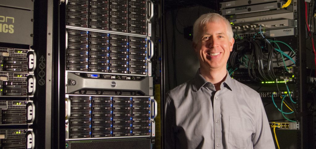
Instructor: Matthew Peterson
Course Description:
Introduction to Unix/Linux (5 weeks @ 2 hrs per week)
Logistics:
Date & Time: Sep 25 – Oct 23, Mon/Wed 2:00pm – 2:50pm
For credit: BDS599 CRN 20579
Workshop Cost: $250
This module introduces the natural environment of bioinformatics: the Linux command line. Material will cover logging into remote machines, filesystem organization and file manipulation, and installing and using software (including examples such as HMMER, BLAST, and MUSCLE). Finally, we introduce the CGRB research infrastructure (including submitting batch jobs) and concepts for data analysis on the command line with tools such as grep and wc.
Command-Line Data Analysis (5 weeks @ 2 hrs per week)
Logistics:
Date & Time: Nov 4 – Dec 4, Mon/Wed, 2:00pm – 2:50pm
For credit: BDS599 CRN 20580
Workshop Cost: $250
The Linux command-line environment has long been used for analyzing text-based and scientific data, and there are a large number of tools pre-installed for data analysis. These can be chained together to form powerful pipelines. Material will cover these and related tools (including grep, sort, awk, sed, etc.) driven by examples of biological data in a problem-solving context that introduces programmatic thinking. This module also covers regular expressions, a useful syntax for matching and substituting string and sequence data.
Q1: What do you hope students gain from this workshop?
My hope is that students come to appreciate the power and flexibility of using the text-based command-line interface to interact with (Linux) computational infrastructures. With practice students will become self-sufficient in utilizing the infrastructure to conduct their own research.
Q2: Favorite topic in your course?
Pipelines! The ability to chain the inputs and outputs of multiple commands to filter data is immensely powerful.
Q3: Who should register for this course?
From the first page of the course syllabus: “Linux/Unix Commands, Bioinformatics Utilities, Computational Infrastructure: If you know nothing about the above, then you are exactly in the right course! WELCOME!”
Q4: Advice for users new to bioinformatics and/or programming?
Practice, practice, practice! Learning how to use the command-line effectively is like making a clay pot, you need to get your hands dirty!
RNA-Sequencing (10 weeks @ 2 hrs per week)
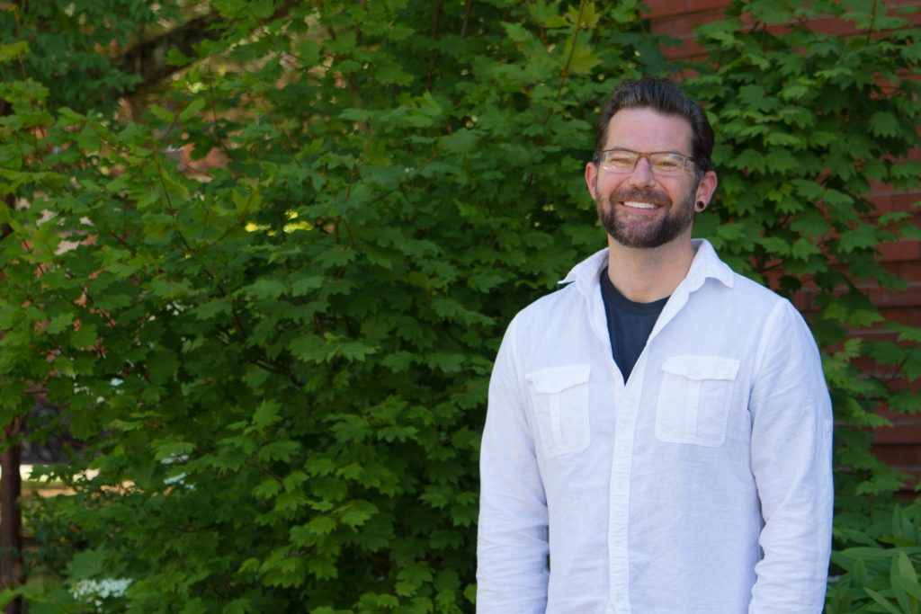
Instructor: Dr. Andrew Black
Course Description:
Logistics:
Date & Time: Sept 25 – Dec 5, Tue/Thur 11:00am – 11:50am
For credit: BDS 599, CRN 20581
Workshop Cost: $500
This course provides an introduction to, and practical experience with, the computational component of bulk-RNA-sequencing. After a general overview, participants will obtain a working introduction to command line, R-studio, and accessing and utilizing a computing infrastructure. Students with then work through a series of exercises cleaning raw FASTQ files, aligning reads to a reference genome, quasi-mapping reads to a transcriptome / de novo assembly, followed by data visualization and Differential Gene Expression analysis.
Q1: What do you hope students gain from this workshop?
I hope that students gain an understanding of the computational workflow involved with RNA-seq and an appreciation of the methodology! My overarching goal with this course is that people can use material from this course as scaffolding for analyzing their own data on the CGRB infrastructure.
Q2: Favorite topic in your course?
I added a lord of the rings theme to my course; students are looking for differentially expressed genes between hobbits and golems. I’m a dork, I know, but I had fun spiking different genes into the data and enjoy having students visualize this.
Q3: Who should register for this course?
Graduate students, postdocs, faculty, or anyone outside of OSU that are interested in receiving an introduction to RNA-seq or for those that are needing to learn the workflow for their own project(s).
Q4: Advice for users new to bioinformatics and/or programming?
Take it one step at a time and get comfortable with several commands before expanding your scope. Also, record your commands / code in a text document, because if you aren’t using it on a daily basis, you’ll forget it!
Data Programming in R (6 weeks @ 3 hrs per week)
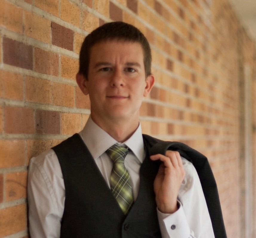
Instructor: Dr. Shawn O’Neil
Logistics:
Date & Time: Sept. 25 – Nov. 6, Mon/Weds/Fri 9:00am – 9:50am
For credit: ST 599, CRN 17196
Workshop Cost: $500
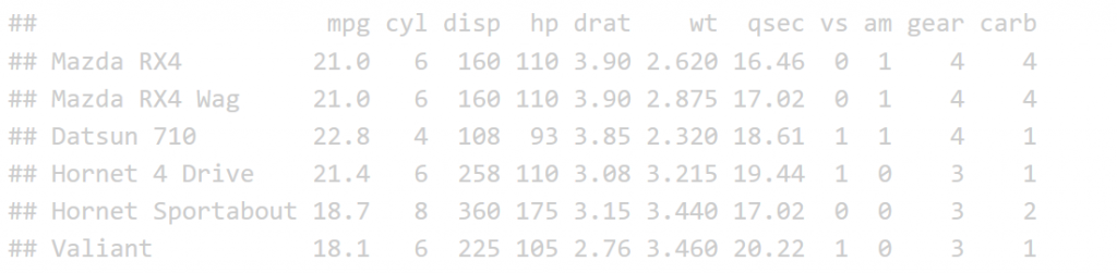
The R programming language is widely used for the analysis of statistical data sets. This course introduces the language from a computer science perspective, covering topics such as basic data types (e.g. integers, numerics, characters, vectors, lists, matrices, and data frames), importing and manipulating data (in particular, vector and data-frame indexing), control flow (loops, conditionals, and functions), and good practices for producing readable, reusable, and efficient R code. We’ll also explore functional programming concepts and the powerful data manipulation and visualization packages dplyr and tidyr, and ggplot2.
Q1: What do you hope students gain from this workshop?
I really hope that students gain an appreciation for programming as a creative activity. It’s not just a means to an end, even with a statistical language like R; there’s a lot of room for play and exploration. Simulation, for example, is a great way to explore complex systems and ask ‘what if’ questions. Many languages (including R) support programmatic drawing and data visualization which can be quite fun.
Q2: Favorite topic in your course?
I always enjoy the point when we first start scaling analyses to thousands of statistical tests. It’s an eye-opening moment, and doing so in R introduces ‘functional programming,’ a powerful and increasingly important paradigm for software design.
Q3: Who should register for this course?
Anyone who is interested in doing data analysis, especially of a statistical sort. For those interested in learning programming in a broader sense, our winter Intro to Python series is an excellent overview of fundamental concepts. Although we cover the same topics in the R course, R organizes its features differently than most mainstream programming languages like Python, Java, and C++. Learning both Python and R provides a solid foundation for data science!
Q4: Advice for users new to bioinformatics and/or programming?
I do recommend learning more than one programming language, eventually, as this helps separate deeper concepts from syntax. Find what motivates you and explore it via programming — this could be your primary research project, some field you’ve been wanting to learn more about, or even a hobby.